

thamerpic
Key points carried forward from May 2022
- Please note that this article primarily analyses LETF Decay (This article is not intended to express a view on likely movements in the Nasdaq or S&P).
- Leveraged ETF decay costs have trebled since the beginning of the year months but now appear to have stabilized, plateaued, and are showing a downward trend (i.e. the cost of LETF leakage relative to their underlying indices is improving)
- In my May June 2022 article, I wrote “Leveraged ETF decay costs tend to be directional: in the absence of any further market shocks, I expect stable (not increasing) LETF decay costs. If markets stabilize or recover, I would expect LETF decay costs to start decreasing from current levels.”
- 2X ProShares Ultra S&P 500 (SSO) will leak only 6% per year (up from 1.5% in February 2022) relative to holding 1X SPDR S&P 500 ETF (SPY) or Vanguard S&P 500 ETF (VOO). SSO still represents a very inexpensive form of gearing/leverage.
- However, 3X Direxion Daily Semiconductor Bull (SOXL) LETFs at current levels, all things being held equal, were in June 2022 set to lose 52% (annualized loss relative to the semiconductor index iShares Semiconductor ETF (SOXX)) of its investment value to decay costs every year (up from 11% in November 2021) .
- Similarly, the short LETFs ProShares UltraPro Short QQQ (SQQQ) and ProShares UltraPro Short S&P500 (SPXU) were very expensive in June 2022, losing nearly 56% (annualized cost) of their investment value per year to costs in current market at June 2022.
- These very costly (in holding cost terms) 3x Semiconductor and Short QQQ (short Nasdaq) LETFs have improved quite dramatically over the last quarter down from 52% and 56% leakage to 37.2% and 34.8 respectively.
- At the beginning of the year, I recommended that “Investors should “De-Risk”: migrate from 3x to 2x LETFS or move into the underlying indices, (to avoid significant costs and underperformance relative to underlying indices) and to avoid LETFs on less liquid indices other than on the S&P500 and Nasdaq100, and avoid short LETFs in those early 2022 market conditions”. Many investors have lost 4/5ths of their investment capital on the high risk LETFs this year through poor market conditions and very high LETF holding costs in sideways markets.
- With LETF leakage costs improving significantly in the last quarter and LETF prices at a fraction of 2021 prices time might be opportune to selectively put a toe back into the LETF market (but only for a small “at Risk” portion of your portfolio that you can afford to lose, and only into low leakage LETFs)
Figure 1: Leveraged ETF “decay” or “leakage” relative to the underlying index and relative to other LETFs for 12 months: October 2021 to date. (Model Source: Author, Data source: Excel 365 Stocks function)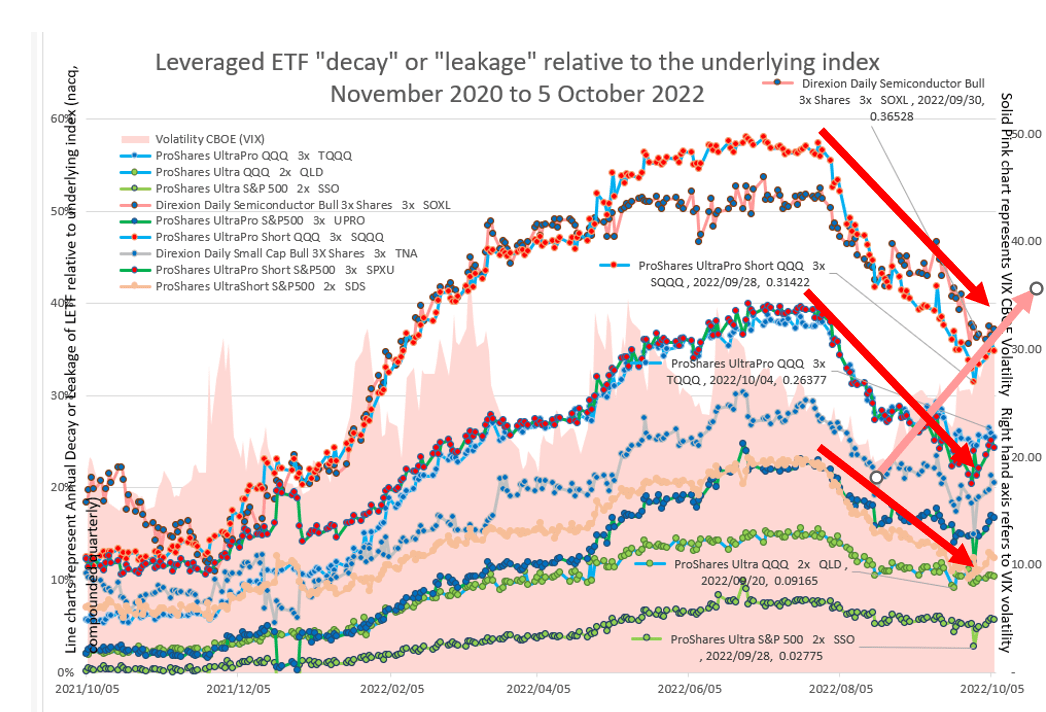
Volatility trending up (pink arrow) while Total Decay on all classes of LETF trending down (red arrows).
3X LETF data analysis:
- ProShares UltraPro QQQ 3X (TQQQ)
- Direxion Daily Semiconductor Bull 3x (SOXL)
- Direxion Daily S&P 500 Bull 3X (SPXL)
- ProShares UltraPro S&P500 (UPRO)
- ProShares UltraPro Short QQQ (SQQQ)
- Direxion Daily Small Cap Bull 3X (TNA)
- ProShares UltraPro Short S&P500 (SPXU)
2X LETF data analysis:
Volatility (VIX) refer pink arrow in Figure 1 is trending down. More on volatility later.
Figure 2: Recent LETF decay trends ranked in the order of increasing decay expense ratios. (Model Source: Author, Data source: Excel 365 Stocks function)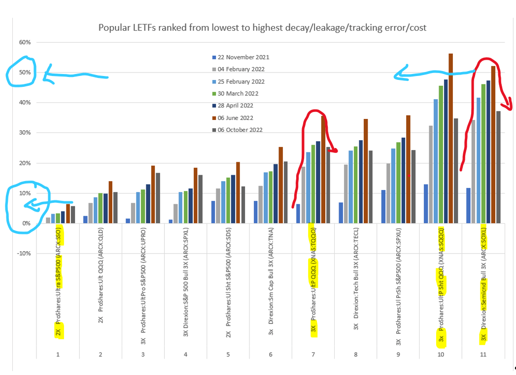
Decay costs have plateaued and are on their way down.
Figure 3: Tabulation of Recent LETF decay trends ranked in increasing order of decay expense ratios. (Model Source: Author, Data source: Excel 365 Stocks function)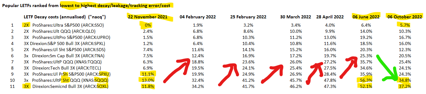
Flat markets allow us to visually corroborate the above mathematically derived data:
Figure 4: Visual observation of ~33% TQQQ degradation (Decay) relative to the Nasdaq Index NDX for the last 2 years, and SQQQ 57% degredation (Source: Data and Chart Source : Yahoo Finance, Annotations: Author))
Decay can be observed visually where index return is flat.
QQQ price movements (green arrow in Figure 4) were flat between 21 September 2020 and 7 October 2022 (2 years). TQQQ underperformed QQQ by 33% over that period (~15.5% decay / underperformance / tracking error per year). SQQQ underperformed QQQ by 57% over that period (~25% decay / underperformance / tracking error per year). These 15%* and 25%* average decay rates per year (over the last 2 years) for TQQQ and SQQQ respectively corroborate the average decay rates used to compile the Decay data in Fig 1,2,3 and 5 above and below. [when markets are flat for QQQ, then the geometric product of all price movement factors over the 2-year period solve to exactly 1. What this means is that any compounding distortions arising from growth in QQQ are eliminated from the TQQQ and SQQQ data over that specific period and any variance between QQQ and TQQQ or SQQQ over that specific period can then only be attributable to Decay (and divergence of the LETFs from QQQ will not be distorted by compounding over that specific period). This visual corroboration is a lot easier than eliminating the effects of compounding mathematically from daily TQQQ and SQQQ price movements, but the results are the same.] [*33% and 57% likewise represent COMPOUNDED decay for 2 years. We also need to eliminate compounding from these numbers to arrive at 15% and 25% annual decay (naca) for TQQQ and SQQQ respectively]. Please observe that SQQQ decays at a significantly higher rate than TQQQ (academically both use the same ^VOLQ volatility inputs). More on that later..
Figure 5: Decay patterns can be highly correlated to one another (they have the same shapes), are highly directional (they move in a consistent direction for some time), periods of high decay appear to lag periods of large price drops (e.g. 2021) and also lag periods of high volatility, and appear to follow a wave or table top pattern., (Model Source: Author, Data source: Excel 365.)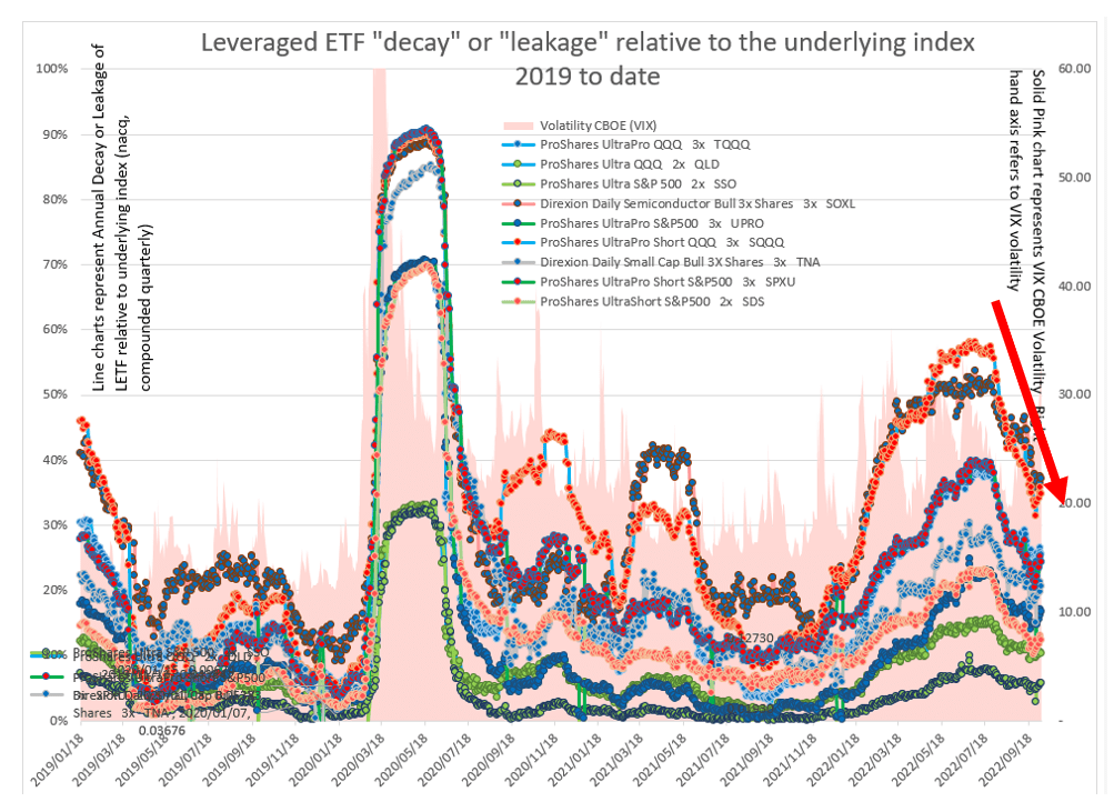
Buy the index (on margin if needs be)
- The alternative to very high leakage LETFs is to purchase the unleveraged ETF on margin if needs be in order to benefit from leverage (provided you well understand the finance costs (relative to LETF costs) and your margin account is very well over-collateralised for the very worst calamitous stock price movements conceivable (you don’t want to get margined out / closed out at the bottom of the cycle but some unexpected black swan event). You would need to re-balance your leverage ratio from time to time (leverage ratio gets thrown out by price movements) to replicate the LETF accurately.
USD 9 trillion FEB Balance Sheet
- I remain concerned about the $8.9 trillion FED balance sheet and the impact that a sale of securities and assets of that order of magnitude (or even a small proportion of that) would have on the market. More on that later in the article.
Volatility Decay
- I have also been banging on about LETF “Volatility Decay” academic models and how volatility (although very important in options pricing) would initially appear (in the short term) to have very little bearing on the pricing of Equity SWAP contracts (which make up 2/3rds of the hedging of 3X LETF). So I had initially really been struggling with the term “Volatility Decay”. Swaps are essentially forward/future equity contracts with leverage, and forwards/ futures are not priced using volatility. But Swap re-hedging burdens and costs (SWAP contract haicuts and SWAP unwind haircuts) do bear a relationship to the volatility of markets and this has to do with the amount of re-balancing required ( “re-balancing effort/costs”) the volumes of which rebalancing are very much linked to the compounded effect of 1. price movements (aka “volatility”) 2. the LETF multiple 3. short or inverse LETFs require greater hedging effort and re-balancing than long LETFs, 4 longer timeframe increases leakage, and 5. more difficult to hedge LETFs (eg Semiconductors) leak multiples more than S&P LETFs. These 5 factors definately do compound one another. While I completely agree with the initial “frictionless” part of the Cheng/Madhavan formula, I must admit that I struggled considerably trying to reconcile the Cheng/Madhavan “re-balancing burden” elements of their formula to real world empirical data and results (as evidenced by Figures 1-5 above). I managed to get a solution this weekend, but some of the Cheng/Madhavan assumptions are questionable , outdated. Hedging strategies (per LETF regulatory returns) do not agree, have changed, moved on and are more efficient than those examples cited by Cheng/Madhavan in 2009. More on that later..
Credit Suisse risk in relation to LETFs
Credit Suisse is in trouble with its credit default swaps reaching 3X the CDS spread of Swiss neighbour UBS, and 4X the CDS spread of BNP Paribas, Europe’s biggest bank.
Credit Suisse could be the next Lehman. CS price charts are a good indicator of the market consensus.
Figure 6: Credit Suisse Credit Default Swap Rates are 3 to 4 times those of other Swiss banks (Source: Bloomberg)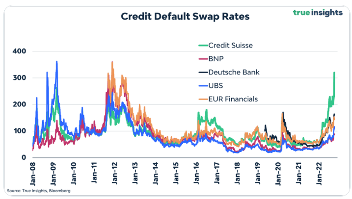
Credit Suisse could be the next Lehman. CS price charts are a good indicator of the market consensus of CS health or distress.
Figure 7: Credit Suisse share price is one sixth of its GFC 2009 low. (Source: Bloomberg)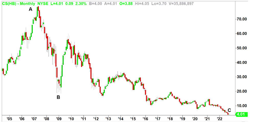
Credit Suisse’s long-term chart is even more disturbing. In April 2007, the stock traded above $79 (point A). After the 2008 crash, Credit Suisse fell as low as $18 (point B). Today, the stock is worth just a fraction (one sixth) of its post-crash price (point C).
The issue here isn’t just Credit Suisse, but other banks as well. As we saw with Lehman Brothers in 2008, financial institutions can be intertwined in incredibly complicated and various ways with massive notional amounts being traded between counter-parties.
In the first week of October 2022, 5.9% of TQQQ’s NAV comprised Credit Suisse Total Return Equity Swaps:
Figure 8: Credit Suisse Total Return Equity Swaps comprised 5.9% of TQQQ balance sheet at beginning of October (Source: Proshares Regulatory disclosures, Yahoo Finance)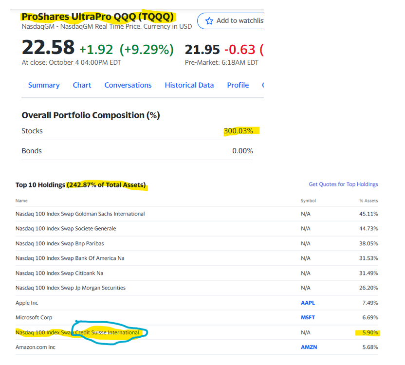
Understanding a Total Return Equity SWAP
For our purposes, a Swap can also be conceptualised as a 2-sided financial contract where the issuer (ProShares TQQQ) borrows $30bn from Bank (“borrowing leg”) to invest in $30bn Nasdaq-100 Invesco QQQ ETF (QQQ) Contracts For Difference issued by Bank (“equity leg”). All of this is usually neatly wrapped into a one-page confirmation contract, signed by both parties.
So, the TQQQ balance sheet has ~$10bn of TQQQ commitments (Net Asset Value) hedged by ~$30bn Equity + ~$20bn of fixed Swap “synthetic” borrowings giving TQQQ a theoretical 3x performance over QQQ.
For those interested, (as cited in my initial article) I think that a traditional Swap contract might look something like my draft below (my drafting entirely). Understanding the possible form of the Swap contract is useful in trying to understand the likely risks embedded in Credit Suisse defaulting.
Figure 9: Example of a Total Return Equity Swap (Source: Author)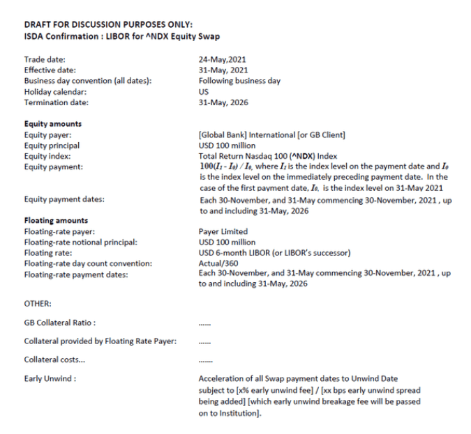
Please note that the following Index or Equity swap should not be confused with a Credit Suisse Credit Default Swap (which is a gauge of CS’s likelihood of default).
TQQQ’s exposure to CS Equity Swaps will depend on a number of known and unknown factors:
At the time of my initial draft: We know that TQQQ has 5.9% of TQQQ NAV exposure to CS Equity Swaps.
Please bear in mind that the SWAPS would comprise a basket of swaps all with different maturity dates, ^NDX exposures, interest rates exposures.
The borrowing leg of the CS Equity Swaps may (would probably) be referenced to short term variable rates of interest (in which case the Swaps have limited interest rate risk), or may be referenced to longer term interest rates (in which case interest rate risk on the CS Equity Swaps will increase if this leg of the SWAP is “out of the money” for LETF Issuer).
The term of the SWAP: Swaps are OTC instruments are oftentimes bespoke (non-standardised) and are difficult to trade out of in adverse market conditions. This applies more particularly to very long dated (say 5 year swaps) than swaps which mature or unwind in say a couple of months. The 2015 movie “The Big Short” provides an interesting overview / helicopter view / refresher on the operation of the swap market and its illiquidity in times of market distress: The are 3 types of market: Bull Markets, Bear Markets and Own Markets.. In an Owl market: you phone Bank / Swap Counter Party and tell him to sell and he responds “Too Whooo, Too Whoo, Too Whoo”.
The “In-The-Moneyness” of ProShares 5.9% of NAV Swap exposure to CS: If CS owes net money to LETF Issuer on these swaps then be worried: This is a direct obligation from CS and that obligation could sit on the CS balance sheet and be subject to a very messy and lengthy compromise and unwind. However if Issuer owes money to CS (a possible scenario if the SWAPS were entered into at a high TQQQ price of $90 (QQQ price of ~$400 or ^NDX equivalent) and now sitting at TQQQ price slightly above $20 ( (QQQ price of ~$300 or ^NDX equivalent) then Issuer owes money to CS and this is less of a problem should CS default (subject to the protections offered to Issuer in terms of the legal drafting of the SWAP discussed below):
The terms and legal framework of the SWAP: Cross collateralisation, set-off and netting provisions of the International Swap Dealers Association (“ISDA”) are intended to regulate the orderly unwind of swaps in the event of an early unwind, a “credit event” (e.g. CS Credit Swap Spreads exceeding multiples of other banks, or CS share price dropping to one sixth of 2008 prices). These ISDA style terms are usually followed in entering into swaps . However big banks (as the SWAP writers) are more often than not able to dictate terms to their counterparties resulting in SWAP terms written very much written in favour of the big banks (and possibly not written in LETF Issuers best interests) on a “take-it-or-leave-it” basis. Hopefully LETF Issuers have entered into these SWAP contracts with eyes wide open and are protected by Netting, Cross-Default and Collateralisation / Cross-Collateralisation provisions of these SWAP agreements, that any exposures are cash settled daily, and that the SWAPs do not have any unwind problems of large haircuts. I have included an example of a publicly available ISDA Swap contract (yellow highlights are mine). Please note that the Bank is usually the SWAP writer (dictating the terms) and that the Bank normally nominates itself as “Calculation Agent” (per footnote 15 of the above SWAP contract). The term “Calculation Agent” appears in this SWAP contract 38 times. In a nutshell the Bank oftentimes gets to dictate unwind basis and all of the myriad of other terms of calculation. We are placing our faith in the LETF Issuers that they have sharp pencils, that any CS exposure is properly collateralised and hopefully immediately cash settled. And hopefully cross collateralisation, set-off and netting provisions apply both to the 2 legs of each SWAP, and also the entire SWAP book between Bank and Issuer. Also all SWAP book exposures are determined in terms of a pre-existing formulaic model or basis and not left to the Calculation Agent discretion which vagueness might lead to pricing uncertainty, disagreement, a sub-optimal unwind in distressed conditions.
It appears that ProShares has reduced its SWAP exposure to Credit Suisse somewhat from roughly 4% of total SWAPS as of October 2021 to roughly 2.4% of the total TQQQ hedging book at present. (It would appear that Swaps are correctly measured and reported at their IFRS-9 Mark-to-Market or “Fair-Value” gross equity value (without off-setting the corresponding debt leg of the SWAP) for TQQQ regulatory return purposes).
Swap Exposures are Labelled “Exposure Value (Notional + GL)” on Issuers’ Holdings disclosures. Presumably “GL” refers to “General Ledger” which I interpret as “In/Out-The-Moneyness” or “SWAP NAV” being carried on Issuer’s balance sheet and possibly not cash settled daily/ regularly. I also see “Net Other Assets/(Liabilities)” of -$8bn which I interpret as Issuer owing Bank on the SWAP (which would make sense in terms of recent market declines). Conclusion : We are trusting that Issuer has adequate safeguards to ensure that these SWAP exposures will not compromised in the event of Bank distress or liquidation.
I am not sure how easy it will be for ProShares to exit their large ~$3billion CS swaps? (again refer the “The Big Short” for liquidity problems in realising/selling OTC Swaps in times of market (or counter-party) distress).
Also consider that TQQQ has used roughly $24 billion Swaps to hedge its TQQQ offering. All of the banks have similar MASSIVE swap positions with each other comprising all the various flavours of SWAPS. Should one of these SWAP counterparties fail, the indirect blowback and contagion to all other market participants will be massive irrespective of any direct exposure to Credit Suisse, and as with Lehman, a domino effect default sequence would likely follow. Measuring Banks’ risk is literally a massively complex task, oftentimes a “black hole”.
The $8.9 trillion Fed balance sheet and Quantitative Tightening
There seems to be some historic relationship between S&P performance and size of Fed Balance Sheet. Both chart overlays have similar exponential shapes and seem to fit. We can shoot holes in the hypothesis firstly past performance is not indicative of future , and secondly high CORRELATIO does not necessarily imply CAUSATION: Reducing the massive FEB balance sheet could continue to have a material impact on markets and suppress markets for quite some time.
Figure 10: Fed Balance Sheet vs s&P 500 (Source: Federal Reserve, Excel Stocks Function)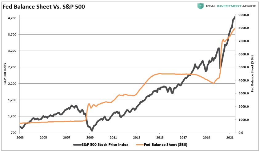
To explain the difference between correlation and causation: Motor vehicle sales, and miles driven also have very similar exponential shaped charts, but we can not assume that motor vehicle sales are driving Fed decisions or are the main cause of stock market price fluctuations. (Similarly Volatility may not be the primary driver or cause of LETF decay (irrespective of any correlations)). More on this later..
Figure 11: Fed Balance Sheet Taper Plan (Source: Federal Reserve, Real Investment Advice)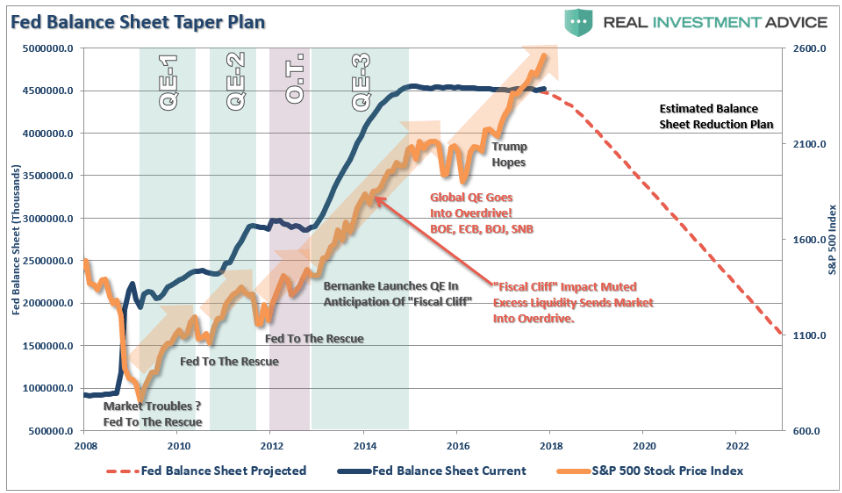
Figure 12: Fed Balance Sheet Taper Plan (Source: Federal Reserve Balance Sheet (Source: Federal Reserve, Wells Fargo),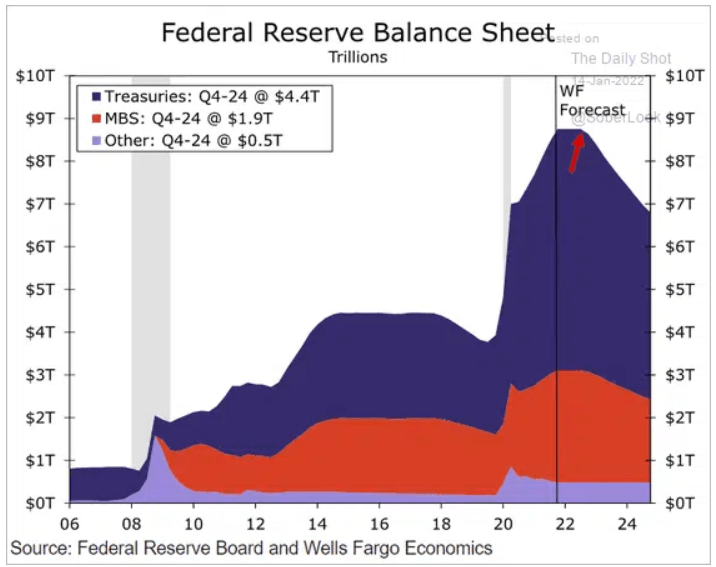
A closer look at the theory of Volatility Decay
Caution: The remainder of this article is targeted at the Quants / Propellor-Heads out there and otherwise may well assist if you are struggling to fall asleep at night.
The following paragraphs are taken (repeated) from my initial LETF article and provide some necessary background:
On page 396 of the TQQQ Prospectus, ProShares cites the following table:
Figure 13: ProShares Volatility and Estimated Fund Returns analysis (Source: ProShares TQQQ Prospectus, Page 394)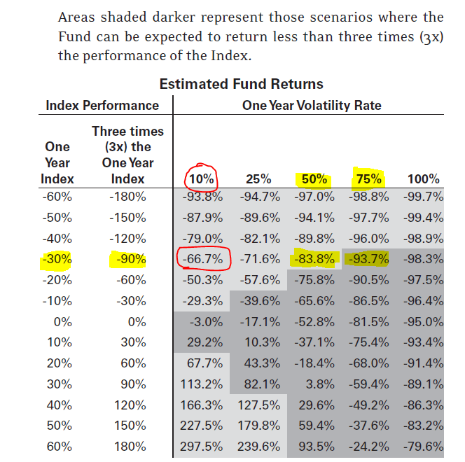
ProShares does not disclose the math behind the grey cells in the Estimated Fund Return % table above. In 2009, Cheng and Madhavan wrote a paper which provides a formula which allows us to solve the above Estimated Fund Returns:
where, in TQQQ’s case: x is the leverage factor of 3 for TQQQ, rx the “Expected Fund Returns” of TQQQ per the greyed cells in the table above, μ is QQQ Nasdaq 100 underlying index expected return (for, say one year), σ the expected standard deviation (annual divided by square-root of days) (which is a proxy for volatility), and tN is the numbe
Figure 14: Cheng Madhavan (2009) Leveraged ETF formula incorporating compounding and volatility (Source: Dynamics of Leveraged ETFs: page 13, formula 25)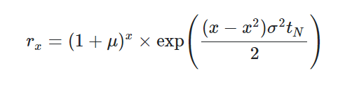
r of trading days (e.g. 252 trading days in a year). The volatility element of this formula uses similar bell-curve-shaped price probability distributions that were used in Black Scholes (1973).
As stated above, I have been banging on about LETF “Volatility Decay” academic models and papers for some time.
Having thought further about this element of the above Cheng Madhavan formula, the volatility implied in this element of the formula is not option-related implied volatility, but is an adjustment to take into account the frequency and magnitude of re-hedging requirements (hedge manager burdens) to re-balance the LETF (TQQQ) in order to maintain a daily (or continuous) 2/3rds hedging ratio) (which re-balancing comes at a “haircut” cost to LETF investors).
We know that continuously entering into and redeeming SWAPS is going to incur SWAP haircut costs on the way in and out. So 1. the more frequently and the larger these “rebalancings occur”, the more the LETF is going to leak oil. 2. We also know that the LETF will leak more oil over a long period than say one day. 3. Thirdly the LETF will leak more oil with highly volatile indices e.g. Semiconductors (compared to less volatile indices e.g. S&P or Russell) because price movements will be greater and re-hedging demands will be greater. 4. Aside from being more volatile, Semiconductors are also more difficult and costly to hedge (less liquid) than say S&P. 5. LETFs will leak more oil in highly volatile market conditions (e.g. the COVID crash) where re-hedging demands are greater than in benign markets. 6. Higher multiple 3X LETFs require exponentially more hedging effort than 2X LETFs and 7. Short / Inverse LETFs require exponentially more hedging effort than Long LETFs.
I use the following frictionless part of the Cheng/Madhavan/Zhang formula extensively in calculating Total decay per charts 1 to 6 above:
Figure 15: Frictionless (Decayless) part of Cheng Madhavan (2009) Leveraged ETF formula incorporating compounding (Source: Dynamics of Leveraged ETFs: page 13, formula 25)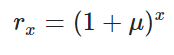
The following element of the above Cheng/Madhavan formula adjusts the frictionless part of the formula exponent to into account “volatility decay”:
Figure 16: “Volatility Decay” part of Cheng Madhavan (2009) Leveraged ETF formula (Source: Dynamics of Leveraged ETFs: page 13, formula 25)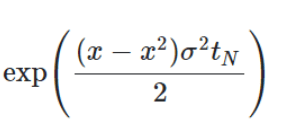
Lets look at a daily re-hedging example. Using the 2009, Cheng/Madhavan element of the formula above: Cheng/Madhavan assumed that $100 2X LETFs were hedged completely using $200 Equity Swaps and by placing $100 into TBonds.
Figure 17: Volatility Decay example cited by Cheng Madhavan (2009) Leveraged ETF formula (Source: Dynamics of Leveraged ETFs: page 13, formula 25)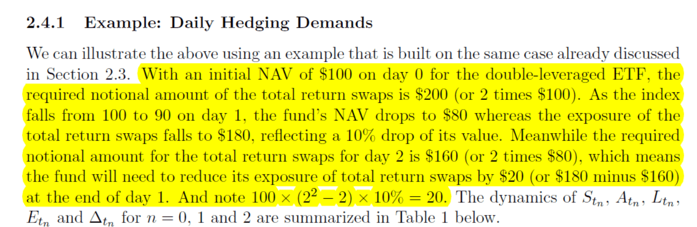
(These hedging assumptions are not correct in terms of current hedging practices: $100 2X LETFs are currently hedged using ~$100 Equity Swaps and by buying a ~$100 basket of stocks (i.e. notional Swap exposure is half of that cited by Cheng/Madhavan, which is a significantly more cost efficient hedging strategy)) , but lets follow the Cheng and Madhavan methodology for now to work through an example. Assuming interest rates, SWAP leverage costs, dividend impact, fees are all zero. .. Also assume that all of the above LETFS are today trading at $100, lets analyse a 5% or $5 price increase in the underlying index per Cheng/Madhavan logic:
Figure 18: Proof of Cheng/Madhavan “re-hedging Burden” X^2-X decay formula for 1X, 2X, 3X, -1X, -2X and -3X LETFs and recalculation of Re-Hedging Burden on the basis of more efficient real-world hedging (using 100% stocks and the remainder of hedges using Swaps) as well as various observations and conclusions in green (Source: Author)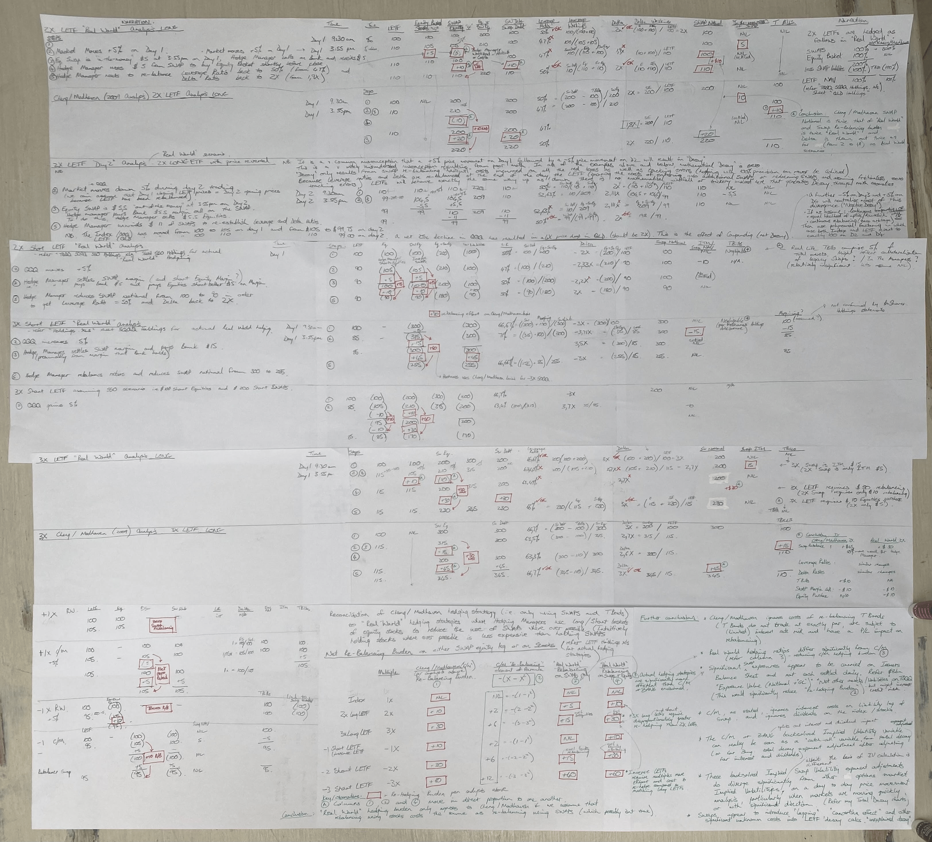
Applying Cheng/Madhaven hedging strategies, a +2X Long ETF with an initial value of $100 starts with a leverage ratio of 50% (ensuring investors a 2X return) at 9.30am on Day 1. (Note: Below is how I envisage the re-hedging. Please comment below if you think my logic is flawed or basis is incorrect). During Day 1, the underlying index moves up +5%. The 2X LETF increases by a $10 price movement (being 2X $5 index price movement i.e. LETF increases from $100 to $110). The SWAP now has $210 value on the equity leg of the SWAP, and $200 on the leverage leg of the SWAP. The SWAP is “in-the-money” by $10 (i.e. SWAP has an NAV of $10). The LETF’s total dollar leverage ($200 SWAP Liabilities less $100 Tbills) remains constant at $100. The leverage ratio has dropped from 50% to $100/$210 = 47.6% and the hedge ratio or “Delta” has also dropped from +2X to +1.9X (refer workings above per Figure 18). Proshares needs to rebalance the gearing ratio from 47.6% back up to 50% in order to assure investors a full undiluted 2X return going forward. To do this (according to my understanding of Cheng/Madhaven method), Hedge manager calls in the $10 “in-the-moneyness” of the SWAP and buys $10 TBills. SWAP now has a NAV of zero. Hedge Manager then increases the SWAP notional by $20 (both SWAP legs increase from $200 to $220). The end result is that Gearing Ratio is restored to 50% and Hedge Ratio or Delta is restored to +2X. Cheng/Madhavan propose that the “total hedging burden” is the net $10 in this scenario (being the net movement in the equity leg of the swap from $210 to $220. Per their “hedging burden” element of the formula: -(2 – 2^2) x $5 price move = $10 “Re-hedging burden”. I would submit that actual real world heding strategy per (refer Figure 19 below: Data Source: ProShares Prospectus, Proshares Web site) is significantly different from Figure 17 above. Hedging Manager doesnt hedge with $200 SWAPS. He hedges with (roughly) $100 Equities and $100 Swaps. 2. But if he did hedge with $200 SWAPS then the “Burden” would be the $20 gross increment in SWAP notional and $10 increment in TBills. (refer first 2X LETF rebalancing examples per Figure 18 above) (In the comments below, Kudos to those with different re-hedging methods or who can write up the +1X, +3X, -1X, -2X and -3X re-hedging methodologies (for +5% index price movement both on the Cheng/Madhavan/ Zhang basis (without using stocks to hedge) on on the Actual Real World hedging strategy basis (i.e. using $100 stocks and the remainder Swaps to hedge). (comments, critiques also welcome including on likely hedging cost differences between these 2 methods)
Figure 19: Proshares LETF Holdings and Hedging Strategies (Source : Proshares website, Hedging ratio calculations per spreadsheet: Source: Author)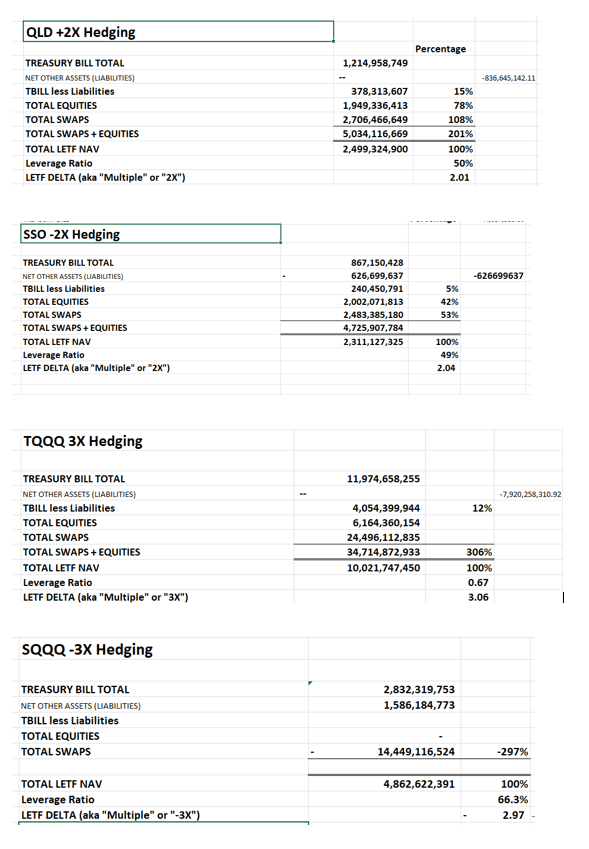
What we do know about the effects of leverage on Decay:
- We know that 3X LETFS require greater SWAP notional than 2X LETFs per LETF dollar: $1bn 3X TQQQ require $3bn hedging whereas $1bn 2X QLD require $2bn hedging.
- Per the Figure 18 analysis above, we also know that in additional to the greater proportion of notional hedging, that in the real world 3X LETFs require a lot more re-hedging per $ of notional than 2X per LETF dollar (relative to the same notional Swap value). i.e. 3X hedging ratios are thrown out more than 2X hedging ratios for the same index price movements (i.e. 3X have higher “gamma” or higher propensity for the 3X multiple to drift).
- So the re-hedging burden is the compounded product combination of 1. x 2. above. i.e. the re-hedging burden from 2X to 3X is disproportionately and exponentially greater.
- And we also know from the above analysis that Inverse LETFs hedging ratios are displaced significantly more for a 5% price movement than Long ELTFs’ and consequently the amount of equity and SWAP equity that requires rebalancing for Inverse LETFs is significantly higher than for Long LETFs. (For Long 2X LETFs, assuming a 5% index increase, Hedge Manager will have to increase the SWAP notional to maintain leverage and hedging (2X delta) ratios by $20 (from $200 to $220): but a proportion of the re-hedging requirement is already taken care of by the increase in the $10 SWAP Equity leg value, requiring a small net rebalancing $10 rebalancing from $210 to $220 in the example above i.e. The Hedge manager is swimming with the current (i.e. re-hedging in the same direction as the index movement).
- Whereas with Inverse LETFs, the SWAP Equity leg increases from $200 to $210, but the Hedge manager requires a decrease in Swap notional from $210 down to $180, requiring a significantly greater (3 times greater) $30 rebalancing effort for the Inverse -2X LETF. The Hedge Manager is swimming (hedging) against the price movement current for inverse LETFs so inverse -2X LETFs naturally leak a lot more oil than Long +2X LETFs, and -3X LETFs leak a lot more oil than +3X LETFs. These relationships are very evident from the Total Decay charts and date per figures 1 to 6 above. Real World hedging strategies however differ from the theory but the principles nonetheless hold although (from the empirical data charts 1-6 above) these relationships hold in a far less formulaic manner, (i.e. actual volatility oftentimes bears very little relationship to the back-solved Swap implied volatility) because Swap leakage can also be driven by other Swap specific extraneous influences (including Swap ‘Lagging”, Swap “concertina” effect, large fund withdrawals/inflows will require Swap unwinds/adjustments which might trigger Swap haircut/unwind costs/ cost accelerations/cost recognitions well in excess of re-hedging costs, unexpected “Calculation Agent” cost adjustments etc etc..
So from the above actual hedging data per Figure 19 above you can see that in order to be properly hedged:
2X Long LETFs require 100% SWAPS i.e. ~ half the SWAP notional that 3X Long LETFs (200% SWAPS) require.
2X LETF leverage ratios are thrown out by a significantly lower proportion than 3X LETFs’ for the same underlying index price movements.
2X Short LETFs (200% inverse SWAPS) require about the same SWAP notional as 3X Long ETFs (200% SWAPS)
3X Short LETFs require negative 300% SWAPS i.e. ~50% more SWAP notional than Short 2X LETFs (200% SWAPS)
In the real world Swaps are used between 33 and 50% less than contemplated by Cheng/Madhavan/Zhang and $100 TBills per the example above are largely replaced by $100 stocks but the hedging effective is exactly the same (albeit more cost efficient).
My objective is to look at the investment decision of LETFs vs buying the underlying index on margin. I (in part) use the first part of the Cheng/Madhavan/Zhang frictionless part of the formula analyse total decay leakage in the charts 1-6 above, (having isolated out the distorting effects of compounding and index price movements). I don’t try to hyper analyse the minutiae of the other interest, dividend of total decay. Those variables are known. I remain unconvinced about the usefulness of the Swap Volatility Decay variable for LETF investment decision making purposes which still leave a large slug of “unexplained decay” variables and discrepancies on the table. (I prefer to look at “total decay” costs). It is relatively easy to isolate out interest and dividend factors from my “total decay strips”, but I haven’t looked at this as yet as these as yet because the total picture is more important to me and my investment decisions at this stage.
The Zhang model:
Figure 20: Zhang model incorporation Cheng/Madhavan decay formula as well as interest on borrowing leg of Swap to solve for “Unexplained Variances” between modelled and true LETF prices for TQQQ. Note Unexplained Variances spiked considerably from practically zero in MArch 2020 periods of very hgh 80% Nasdaq VOLQ volatility (Source: University of Cape Town Actuarial Science Dept)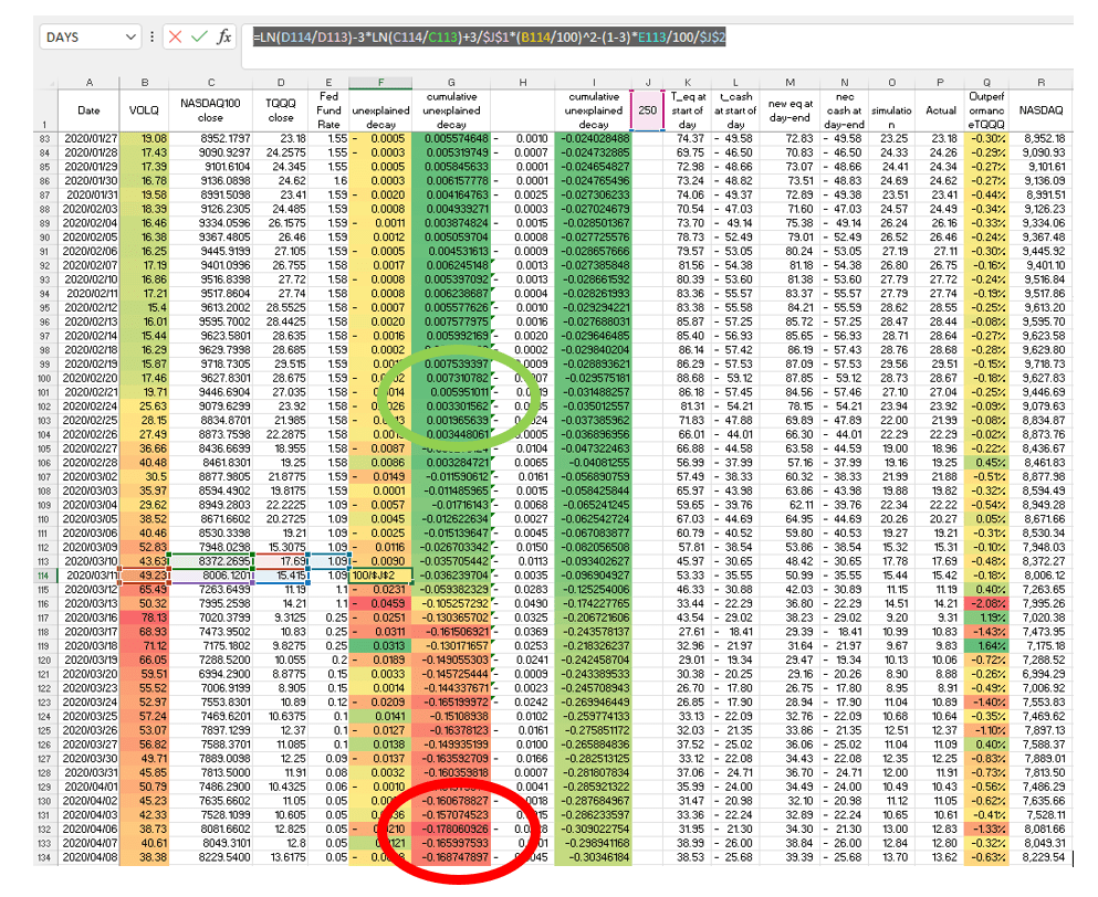
The above spreadsheet was very kindly contributed by Erich Maritz and his team: School of Actuarial Science and Management Studies: University of Cape Town. This model is (as far as I am able to understand the math) based on the following Zhang paper: (heatmaps / color scales are mine). Please note that the Zhang model separately seeks to isolate the impact of volatility aka “re-hedging burden/costs”, interest rates, dividends, disclosed issuer fees, whereas I am more interested in Total Decay aka “total leakage / tracking error” away from the index for investment / trading decision making purposes per my decay charts above. Both models use the same / very similar math / logic. (please refer previous articles for my heatmap modelling over the March 2020 period) The ZHANG model does hold true in periods of low volatility (when the impact of volatility on the model outcome is exponentially lower). However my point about volatility models not always being accurate is very well illustrated by the excel spreadsheet over the March 2022 period: Refer “cumulative unexplained decay” The “cumulative unexplained decay” changed from practically zero (green highlighted circle) to a very large variance (red highlighted circle) within a matter of days between end of February 2020 to mid march 2020. Stated differently, the volatility models might work adequately in very low volatility periods (when the impact of the volatility component of the formula is very low) but all volatility models failed to produce useful theoretical pricing for TQQQ during March 2020. (refer my theories on carry forward of legacy SWAP costs/benefits and SWAP concertina effects above, and market price movements do not always follow perfectly bell shaped pattern) I think that we can safely conclude that the volatility based formulae diverged significantly from actual TQQQ pricing during March 2020, and this failure corresponded to times of highest volatility when the volatility component of the formula had a much higher impact on pricing. So actual vs theoretical TQQQ correlations would be thrown into disarray during periods of very high volatility (and Erich seems to agree with me on this). For the beginning period of March 2020 back-solved TQQQ volatility averaged out at practically zero whereas VOLQ spiked up to 80% during that period. The excel formulae have been included for those interested in re-modelling..
A quick look at another form of Volatility asymmetry
Figure 21: Daily Nasdaq Price Movements (Variances) over time show narrowing of Daily Variances in last 3 months despite upward trend of VOLQ Nasdaq volatility (Source: Model Source: Author, Data Source: Excel 365 StockMarket Functions)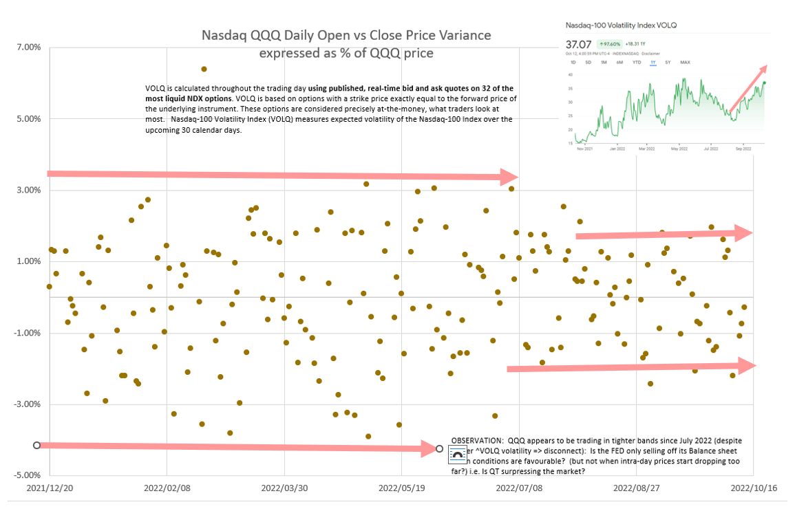
Lastly, I look at previous day price movements early every morning over coffee. Daily price movements seemed lower than previously. That got me wondering whether the Fed (or some other very powerful party) was selling , but only selling and selling heavily when daily price movements were above say positive 2%, and then withdrawing all sell orders when the market was heading into negative territory. Because that is how I would try to sell if I had a 9 trillion dollar balance sheet to get rid of without destroying the market. The above is a scatterplot of daily price variances on the Nasdaq 100 over time. Daily Nasdaq price movement variances seem to have narrowed to a tighter band since July 2022. However the Nasdaq-100 Volatility Index (VOLQ) (chart inset at top RH corner) is trending upwards which doesnt seem to make any sense at all. Nasdaq volatility is admittedly measured on a different basis: “Nasdaq-100 Volatility Index measures 30-day implied volatility as expressed by the prices of certain listed options on the Nasdaq-100 Index (NDX) to obtain the prices of synthetic precisely at-the money (ATM) options.”
Be the first to comment