3D Volatility Ratios For Investment Decision-Making

The Legend

For the past year or so, my research has centered on market volatility. For example, Trading Secrets Of The Toltecs from September 2021 and Fifty Shades Of Deviation from October.

Volatility is the most difficult problem in finance, so studying it seemed like a good way to evaluate the soundness of my analytical framework. The framework is designed to facilitate market insight, so it would be nice if it actually does that.

This article will outline a very simple volatility analytical methodology that may have some theoretical academic importance.

EWMA Volatility Numbers

In finance, volatility (usually denoted by σ) is the degree of variation of a trading price series over time, usually measured by the standard deviation of logarithmic returns.

How To Make A Stochastic Volatility Supermodel showed why the broad academic consensus is to measure volatility with an EWMA (exponentially weighted moving average). EWMA resolves fixed time segmentation issues associated with the classical standard deviation equation. EWMA numbers are demonstrably more accurate with the huge added benefit of being much easier to calculate.

The EWMA calculation is very similar to the EMA (Exponential moving average) which is a universal feature on all commercial charting platforms. I’m not aware of any platform calculating EWMA, a situation that seems somehow sad and pathetic.

Calculation Logic – Close Deviation

Jen: If you can take back the sword in three moves, I’ll go with you.

– Crouching Tiger, Hidden Dragon

Supermodel complained that all of the dozens of otherwise excellent YouTube videos on EWMA do not clearly explain how to code the calculation. Since the solution is only a few lines of code, I’m hoping the explanation below is useful.

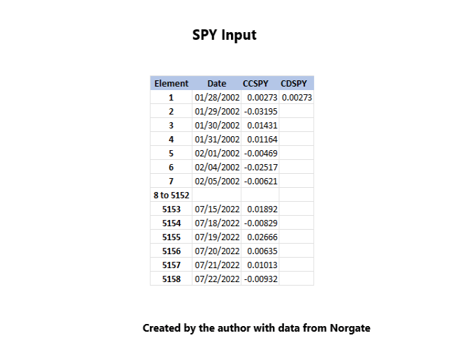
My research begins after converting a stock’s price history into daily logarithmic returns. Open, High, Low and Close prices are discarded after an initial build step.

CCSPY is the daily logarithmic return. CC stands for Close to Close.

CDSPY is the EWMA of CCSPY. CD stands for Close Deviation

The Element column isn’t visible in real life, it is simplest to think of it as a row number. For example CCSPY(1) = 0.00273

A single work variable (CCVAR) is used to keep track of the EWMA quasi sum of variances. This is much cleaner and more efficient than the classical calculation, which requires each day’s variance to be stored as an array element before summing when doing historical analysis.

CCVAR = CCSPY(1) ^ 2 (CC squared)

CDSPY(1) = CCVAR ^ 0.5 = 0.00273 (square root of CCVAR)

The calculation for subsequent CDSPY values is based upon a weighting parameter represented by the Greek letter Lambda. Lambda is a number between 0 and 1 that controls measurement sensitivity.

In this article, Lambda = 0.95. 1 – Lambda = 0.05 indicating that the current day’s variance is weighted at 5%.

To calculate CDSPY(2), CCVAR currently has a value of CCSPY(1) ^ 2:

CCVAR = (CCVAR * Lambda) + ((CCSPY(2) ^ 2) * (1 – Lambda))

CDSPY(2) = CCVAR ^ 0.5

The logic for all the elements from 2 until the last is exactly the same so populating all the rows is very quick and simple with a For Loop:

For x = 2 to 5158

CCVAR = (CCVAR * Lambda) + ((CCSPY(x) ^ 2) * (1 – Lambda))

CDSPY(x) = CCVAR ^ 0.5

Next x

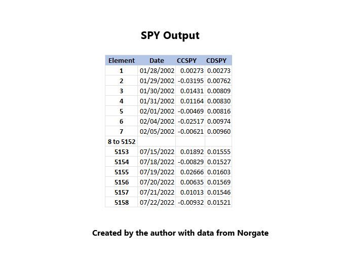
The early numbers in a sample will not be totally kosher until a certain number of observations have been processed. The exact number of early observations that (maybe) should be discarded can be calculated, but ignoring the first 100 observations, for example, is safe.

Volatility Dimensionality

After cursory analysis, two volatility dimensions are obvious. They can be accurately measured by:

• CD, Close Deviation; and
• RD, Range Deviation.

Range Deviation

It’s not easy to believe, but my suggestion to calculate standard deviation for the daily range might be original. The typical technical indicator for Range is the average true range. That number is useful for very short term risk quantification. Otherwise, like all technical indicators, it is kind of lame and feeble.

Financial statistics dismisses range as “noise.” That position made some practical sense before the invention of computers. I’m hoping my research changes some attitudes, but whatever.

The RD calculation has been changed and hopefully improved in this article. Daily range = High – Low. True range substitutes the previous close in the formula if it is higher than the current daily high or lower than the current daily low. This article will consider true range.

For Range to be analytically useful it must be normalized, for example:

• Range = (High – Low) / Previous Close

I decided this number is a bit off and changed the calculation to:

• If CC > 0, Range = NatLog (High – Low + Prev Close) / Prev Close
• Else, Range = Natlog (Prev Close – (High – Low)) / Prev Close

That has the effect of introducing negative numbers into the return stream, which gets resolved when the negative numbers are squared in the RD calculation.

RD Calculation

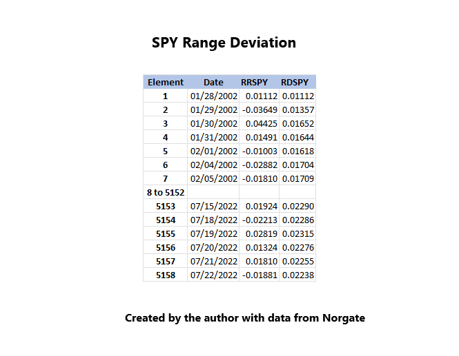
RRSPY is the result of the calculation described above. RR stands for rate of range which is a pun on the term rate of change.

The RDSPY calculation is the same routine as CDSPY except that the input column is now RRSPY.

Toltec Deviation, The Third Dimension

Intuitively, a third dimension of volatility should exist, but the nature of it is elusive. I’ve been looking for it for twenty years or so, in between doing some other stuff.

The concept of Toltec trading daemons was introduced in Trading Secrets Of The Toltecs as a viable way to measure volatility. Toltec = Impeccable so Toltecs are always on the correct long/short side of the market through finite states. It has taken about a year to develop that concept into a plausible third dimension solution.

Toltec deviation is based on daily finite state price movements. CC, or logarithmic return for a market day, can be divided into two finite states:

• CO = logarithmic return from Close to Open
• OC = logarithmic return from Open to Close

CC, CO, OC, RR and the daily EWMA numbers are all calculated in the build step.

Toltec Deviation Input

CC = CO + OC

The return stream for Close deviation is CC. An equivalent way to say CC is CO + OC. The return number for Toltec deviation is:

Absolute value CO + Absolute value OC

TD Calculation

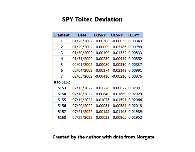
In this case, the calculation involves adding the absolute values of CO and OC, but otherwise the routine is the same as CD and RD.

CDSPY could also be calculated by adding the CO and OC numbers instead of CC.

Major Index And 3X Bull Current Volatility

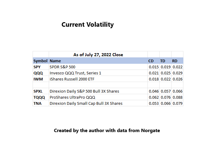
RD is almost always higher than TD, and CD can never be higher than RD or TD. Supermodel went through detailed return / volatility distribution analysis. Probably on account of the abnormal distribution of returns, interpretation of the information presented this way is inherently unreliable.

Beat The Market With Delta Force showed that 3X Bulls (and Bears) are pretty much exactly 3 times more volatile than the underlying. That can be seen in the table above. This fundamental truth is probably the single most critical thing to understand in order to trade these instruments rationally.

Two other important statistical givens (can be proved) that are a bit less momentous are:

• Correlation with the underlying is always very close to 1.
• Beta with the underlying is always very close to 3.

Paying close attention to Major Index 3X Bulls, is an excellent way to understand the current market environment. If nothing else, the numbers are a lot more interesting to look at than the underlying.

In this article, TQQQ will be looked at.

Abnormal Distributions

Frederick Frankenstein: Are you saying that I put an abnormal brain into a seven and a half foot long, fifty-four inch wide GORILLA?

Young Frankenstein

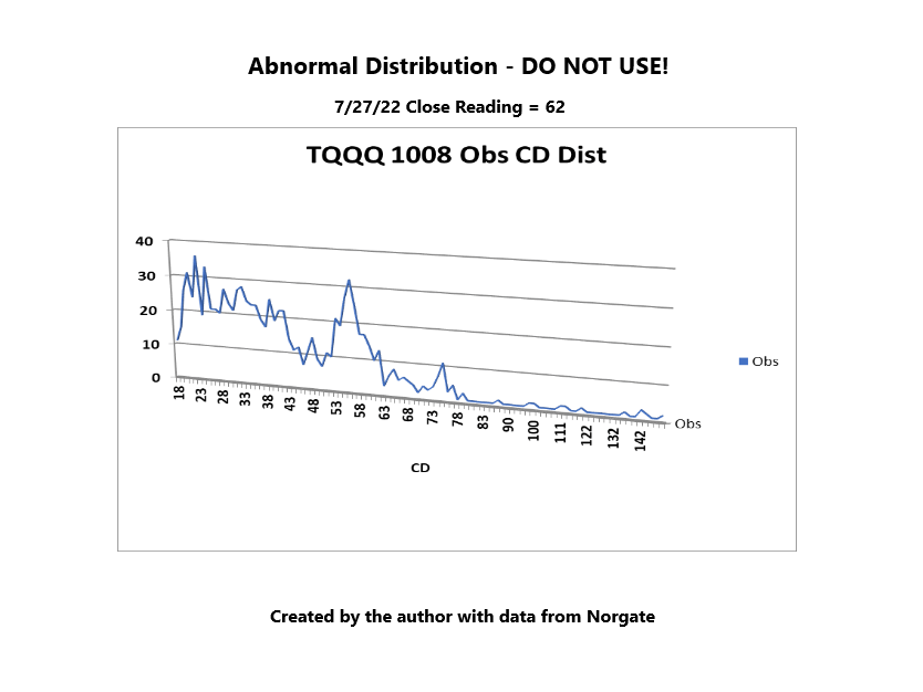
The numbers along the bottom are the observed CD Numbers multiplied by 1000 and stored as integers. The integers are important because they can be used as element numbers. This simple technique to resolve binning issues was also used in Supermodel.

The 7/27 reading of 62 – 0.062. The current reading is very close to the start of the right tail. The obvious message is that things are dangerous here, a fact which most rational observers are already well aware of.

Looking at volatility through the raw numbers is not much different than looking at a technical indicator. The term “good technical indicator” is sort of an oxymoron, but raw volatility numbers are unusually poor in that type of application.

After developing the TD and RD dimensional measurement standards presented above, there was a progression in deciding what to do to understand the numbers. Volatility ratios are a result of that investigation.

3 Dimensional Volatility Ratios

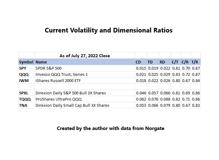
There are three possible dimensional ratios. They are listed below along with the SPY long term 3024 observation medians:

• C/T = CD/TD, 0.80
• C/R = CD/RD, 0.67
• T/R = TD/RD, 0.84

The abnormal nature of single dimensional volatility distributions was shown above. It turned out that the ratios between the three dimensional ratios are normally distributed.

Of course, that was totally unexpected. Personally, my previous guess had been that normal distributions were impossible to create with market data. The academic guys will probably say this is about as profound as the formula for ice cubes, but to me, it is definitely worth checking out.

Normal Distribution

If a distribution is normal, it can be graphed into something looking like a bell shaped curve and after 5 million years or so of evolution, human beings are remarkably good at analyzing that type of pattern. There are several statistical techniques to quantitatively evaluate bell shaped curves, but even the sages recommend looking at the data first.

TQQQ – C/T Ratio

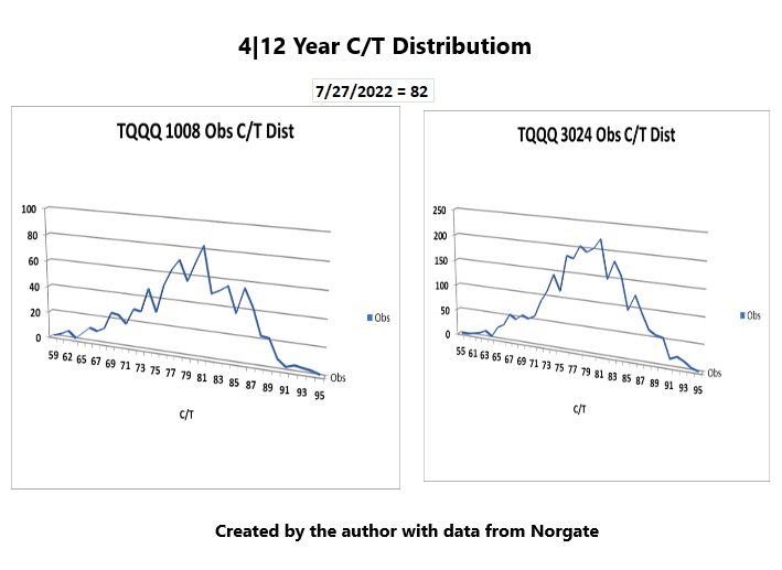
Needless to say, I hope I’m not the only one who thinks these distributions look normal.

The idea is that both long term and short term distributions should both be normal and look about the same, except the short term appears less smooth.

The numbers along the bottom are the observed ratios multiplied by 100 and stored as integers. The current reading is 0.82 * 100 = 82.

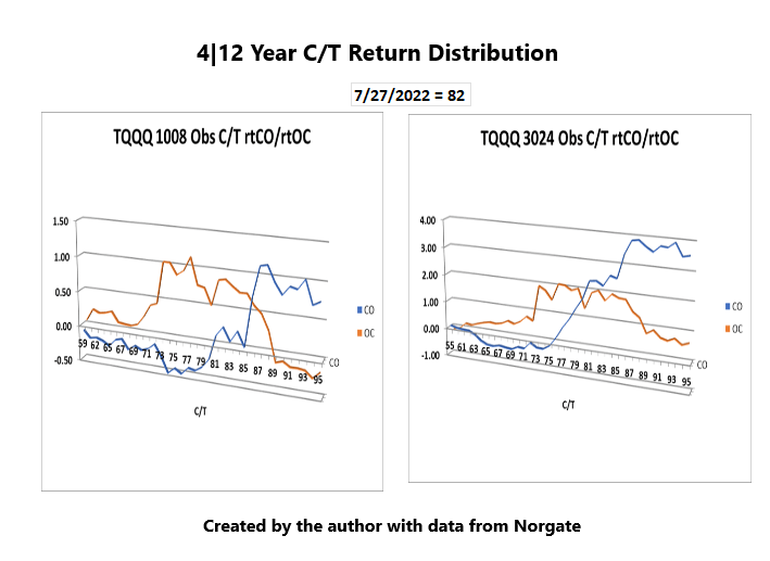
Running return totals are a remarkably good and simple way of looking at returns. When strategists go into their drawdown song and dance, it’s pretty much just running totals. Usually running totals are sequenced by time.

The returns are logarithmic.

I forget which one of these I created first, but I experienced some doubt that the other one would look at all similar.

The pattern of CO weakness coupled with OC strength and vice versa is quite striking. The Yin-Yang pattern is part of the Toltec’s nature.

(‘dark-light’, ‘negative-positive’) is a Chinese philosophical concept that describes how obviously opposite or contrary forces may actually be complementary, interconnected, and interdependent in the natural world, and how they may give rise to each other as they interrelate to one another.

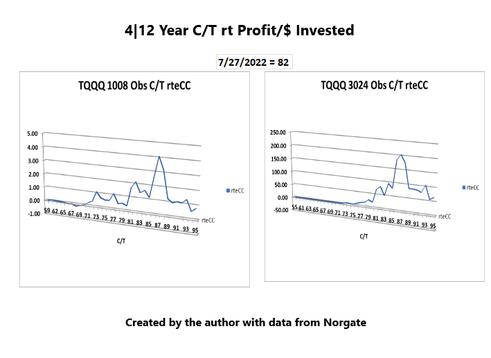
This CC study is running total of profit/$. Even though the current 4 year period is relatively weak the studies are quite similar.

One idea is to try avoiding the drawdown after the ratio peaks in the mid to upper 80s. The peak CC return is 203 times the initial investment at 87, followed by a very sharp drawdown.

TQQQ – C/R Ratio

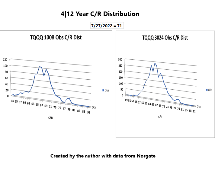
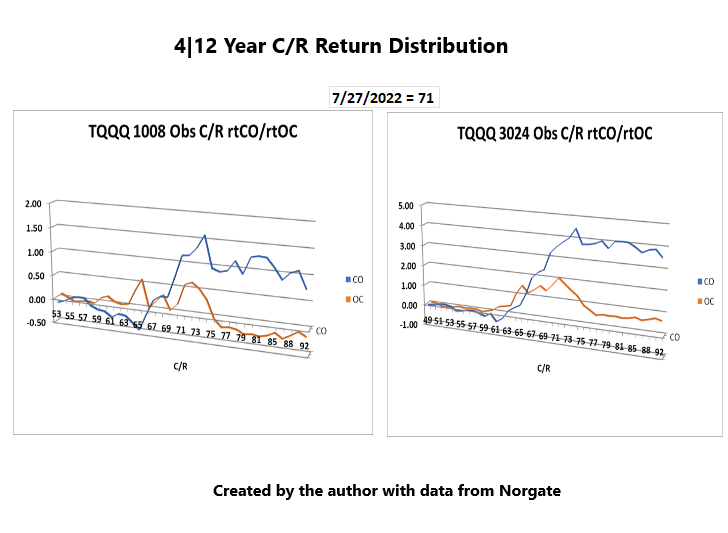
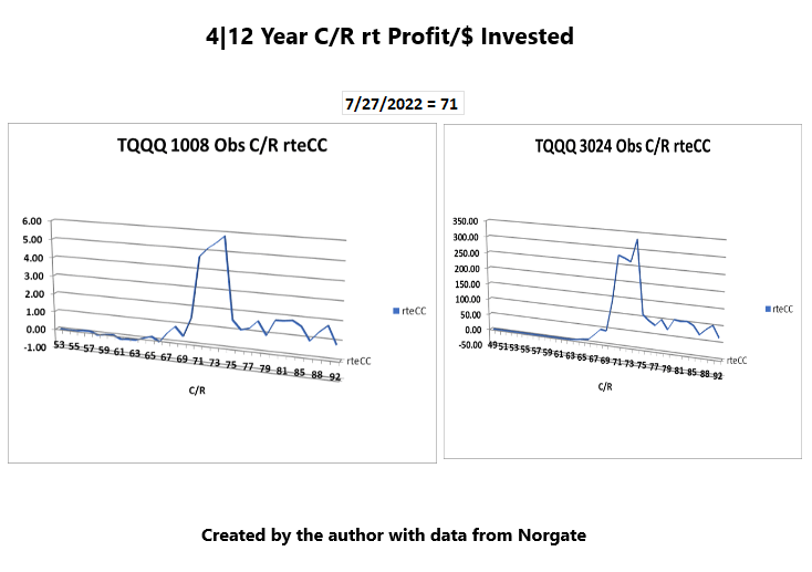
The peak is 331 times the initial investment at a ratio of 74.

A typical computer strategy offsets signals by a day (or period), because it waits for a state transition to change positions. The non-offset return stream is much more important for analytical purposes, so that is what we are looking at here. State transition analysis happens later in the development cycle.

TQQQ -T/R Ratio

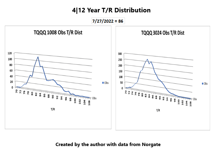
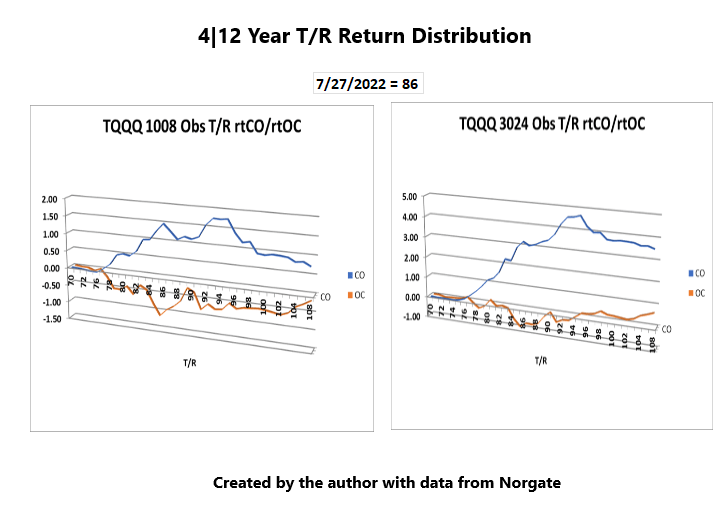
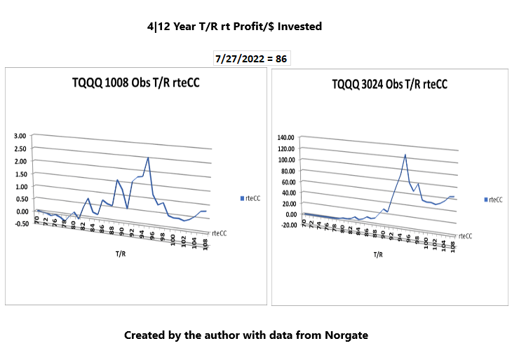
The peak is 126 at 95.

Conclusion

Dimensional volatility ratios seem to provide valuable concrete insights into market volatility that is clearly superior to analyzing the raw numbers. Of course, my view might be a little biased.