This Portfolio Strategy Offers Attractive Returns

By Enrique Zambrano and Carlos Rizzolo

Introduction

In our SSRN paper, we developed a multi-asset momentum strategy that shows attractive risk-adjusted returns and the ability to generate positive returns on a rolling basis while having a low correlation with traditional portfolios. The strategy can be used on a standalone basis or combined with a 60/40 portfolio, enhancing the returns and reducing the volatility and drawdowns. Although the benefits of allocating a portion of the 60/40 portfolio towards the strategy are clear, the combination of the strategy with an all-equity portfolio is worthy of attention. In this article, we analyze if there are significant benefits from combining the strategy with an equity portfolio.

The Strategy

The basic idea is to construct a multi-asset (systematic) momentum strategy. In general, momentum strategies consist in buying past winners and selling past losers. However, since our main goal is to develop a long-only strategy, we focus on selecting the best assets with positive momentum. In this process, we must answer the following questions: which is our asset universe? How do we measure momentum? How do we select the look-back period?

Asset Universe

For the asset universe selection, the focus is to identify assets with ex-ante positive expected returns in at least one state of the economy. In principle, we can characterize economic regimes using two variables (inflation and growth), which gives us four possible combinations.

In a rising inflation/accelerating growth environment, we should expect that Commodities (Energy and Agriculture), Metals, Real Estate and Emerging Markets equities show positive performance. Alternatively, during the falling inflation/accelerating growth regime, we should anticipate that Corporate Bonds (IG and HY), Treasuries, Developed Markets equities and Real Estate exhibit positive returns. On the other hand, when growth slows and inflation is rising, assets such as Cash, Gold and Commodities should behave well. Finally, if growth is slowing and inflation falls, Treasuries should have positive returns. In this sense, our asset universe is composed of the following asset classes and ETFs:

• US Large Cap Equities (S&P 500): SPDR S&P 500 Trust ETF (SPY)
• US Large Cap Equities (Nasdaq 100): Invesco QQQ ETF (QQQ)
• US Small Cap Equities (Russell 2000): iShares Russell 2000 ETF (IWM)
• European Equities: Vanguard FTSE Europe ETF (VGK)
• Japanese Equities: iShares MSCI Japan ETF (EWJ)
• Emerging Markets Equities: iShares MSCI Emerging Markets ETF (EEM)
• US Real Estate: Vanguard Real Estate ETF (VNQ)
• Commodities: Invesco DB Commodity Index Tracking ETF (DBC)
• Commodities (agriculture): Invesco DB Agriculture ETF (DBA)
• Gold: SPDR Gold Trust ETF (GLD)
• Investment Grade US Corporate Bonds: iShares iBoxx $ Investment Grade Corporate Bond ETF (LQD)
• High Yield US Bonds: iShares iBoxx $ High Yield Corporate Bond ETF (HYG)
• Long-term US Treasuries: iShares 20+ Year Treasury Bond ETF (TLT)
• Cash: iShares Short Treasury Bond ETF (SHV)
• Medium-term US Treasuries: iShares 7-10 Year Treasury Bond ETF (IEF)

Furthermore, we segment the asset universe into two components. The first group includes the assets that we will invest in when they exhibit positive momentum (Risk-On universe), and the second group contains the assets that we will hold when the risk-on assets show negative scores (Risk-Off universe). The latter is composed of cash and medium-term treasuries, while the former contains the rest of the asset universe.

Investment philosophy: measuring momentum

Two important elements regarding momentum strategies are the selection of the measure and the look-back period. Rather than running an optimization to identify the best parameters, our philosophy is to combine several measures and look-back periods. We believe that using a single specification would make our strategy more exposed to fortune shocks in the future (both good luck and bad luck). By combining several specifications and considering a bigger piece of the available information, we can build a more robust framework that has higher odds of capturing momentum and less exposure to fortune shocks. Although the framework would probably underperform some specifications in a given time period, we believe that it enhances the prospects for the long run.

In this sense, we use three different measures of momentum and three formation periods, giving us a total of nine combinations. We measure momentum using 1) past total returns, 2) the difference between the price and a simple moving average, and 3) adjusting the past total returns by the sum of absolute daily movements (with the purpose of penalizing assets with “inefficient trends”). All these measures are then adjusted for the correlation of each asset with the risk-on asset portfolio (equally-weighted), favoring assets with low correlations. Furthermore, we use medium- and long-term look-back periods, including 3, 6, and 12 months (50, 100, and 200 days for the moving average). All these combinations provide useful information for our asset allocation decision.

Implementation

The implementation of the strategy is as follows:

1. We evaluate the momentum signals for each asset on the last trading day of each month. Using all the signals, we construct a momentum ranking.
2. We select the top 5 assets in the ranking.
3. We determine the allocation to these 5 assets by considering the number of assets with negative momentum, using the following formula: % Risk On Exposure=max⁡(1-n*4/39,0%), where n is the number of assets with negative momentum and N is the number of assets in the risk-on universe. Once the Risk-On exposure is determined, we assign an equal weight for each of the 5 assets. If the Risk-on exposure is less than 100%, we allocate the rest of the portfolio to the risk-off asset with the highest ranking.
4. If any of the top 5 assets exhibits negative momentum, it is substituted by the risk-off asset with the highest ranking.
5. We hold the portfolio for one month and repeat the process.

Combining the Strategy With an All-Equity Portfolio

We are interested in combining the strategy with an all-equity portfolio. For this reason, we perform a backtest using daily observations from Dec. 31, 2003, to Sept. 30, 2022. The data was retrieved from Bloomberg. The time series are based on total return indexes constructed from each ETF in the asset universe. However, since some ETFs have a more recent inception date, we complete the backtest using the total return of the respective underlying index. For the equity portfolio, we use as a reference the SPY.

We analyze several combinations of the strategy with the equity portfolio. The results are displayed in the following table and chart.

Table 1: Combining the strategy with SPY

	Total Return	Annual Return	Volatility	Ret/Vol	Max DD
Strategy	384.53%	8.79%	8.11%	1.08	-10.29%
SPY	361.68%	8.51%	19.29%	0.44	-55.20%
90% SPY/10% Strategy	377.83%	8.71%	17.59%	0.50	-50.41%
80% SPY/20% Strategy	391.30%	8.87%	15.94%	0.56	-45.30%
70% SPY/30% Strategy	401.84%	8.99%	14.34%	0.63	-40.02%
60% SPY/40% Strategy	409.24%	9.08%	12.82%	0.71	-34.46%
50% SPY/50% Strategy	413.37%	9.13%	11.41%	0.80	-28.86%

Click to enlarge

Source: Own calculations based on data retrieved from Bloomberg.

Chart 1: Growth of $100 (Dec. 31, 2003 – Sept. 30, 2022)

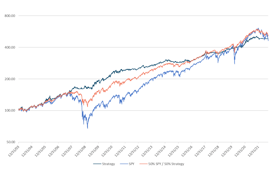
First, comparing the strategy with the equity portfolio, we can appreciate that the strategy experienced similar returns (slightly higher) to the SPY. However, the volatility was reduced by more than a half and the maximum drawdown was less than a fifth. In other words, the strategy shows the potential for equity-like returns but significantly improves the risk metrics. Moreover, the combinations result in higher annual returns and lower volatility and drawdowns. For instance, the 50/50 combination increases the annual returns by more than 60 bps and, more importantly, reduces the volatility by 788 bps while the maximum drawdown is cut in half. In general, combining the equity portfolio with the strategy results in significant benefits for the portfolio.

In chart 1 we can appreciate the return over the entire study period for the strategy, the equity portfolio and the 50/50 combination. We must highlight several important facts. First, the dark blue line (corresponding to the strategy) looks like a straight line; although in some instances it is flat, it has very low downside volatility. The linearity of such a curve suggests that the strategy gives a very stable return stream (note the logarithmic scale). Moreover, during bear markets (for example, the 2008 financial crisis, March 2020 and 2022), the strategy had minimum declines (in reality, it remained practically flat). This uncorrelated behavior implies that one can take advantage of a timely rebalance, boosting the compounded annual growth rate in the long run.

Combining an equity portfolio with a strategy with such characteristics results in a more stable growth. What if we could tell you that, over the long run, you’ll have the same returns of an equity portfolio but with significantly less risk? It definitely sounds attractive, but we must emphasize that it doesn’t come without a cost. Although in the long run the returns are very similar, there are some periods where equities will outperform the combination. For instance, we can appreciate that during the 2010-2019 period, the SPY closed all the gap that was created during the financial crisis. During prolonged bull trends, equities will have higher returns than the combination since the strategy often takes a defensive stance.

Correlation

Combining the strategy with an equity portfolio boosts the returns while significantly improving volatility and drawdowns. The main reason behind this behavior is the diversification potential given by the strategy. To gain more insight, we explore this feature in the following chart.

Chart 2: Three-year rolling correlation between the strategy and SPY

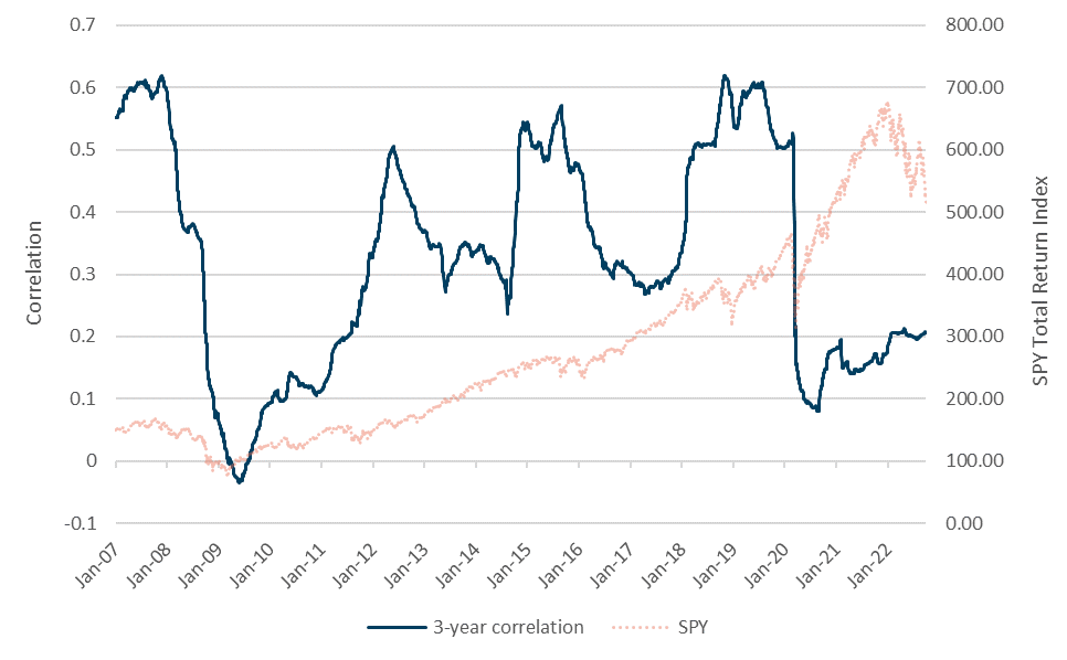
The 3-year rolling correlation ranges between 0 a 0.60, with a concentration inside the 0.2-0.5 interval. The average correlation in the whole period is 0.32. Moreover, the correlation dynamics are quite interesting. The value tanked to zero during the 2008 financial crisis and became small during the 2020 pandemic; in other words, the strategy switched to assets uncorrelated with equities and avoided those big drawdowns. Additionally, the correlation coefficient remained somewhat elevated between 2010 and 2020, capitalizing on the rising trend of equities. In this sense, the overall correlation is small and dynamically adapts to the movements in the stock portfolio. For this reason, adding the strategy to an equity portfolio would provide diversification benefits and enhance returns.

Conclusion

Equities have and may continue to be the asset class with the highest return potential in the long run. We will not make efforts to challenge such a claim. However, we believe that the path is as important as the destination. Equities may suffer big and prolonged downturns, which represent a significant risk for investors. Trying to avoid or minimize such periods should be a priority. In this sense, we present a strategy that can help a stock portfolio preserve its return potential while reducing risk.

There are enormous benefits from combining an equity portfolio with a low-correlated multi-asset strategy. Returns may be marginally improved, but the volatility and drawdowns are significantly reduced. In this sense, we believe that equity investors should consider allocating a portion of their portfolio towards multi-asset strategies.