Goehring & Rozencwajg Q2 2022 Natural Resource Market Commentary

WHY RESOURCES DURING A RECESSION

Over the last two months we have spent a lot of time traveling throughout North America and Europe, speaking with clients about what role natural resources investments should play in their portfolios. During our travels we were also gauging demand for our potential Undertakings Collective Investment in Transferable Securities (UCITS) fund. At these meetings, we learned first-hand what our investors worry about the most. Recession fears loom large.

Investors firmly believe inflation has gone from transitory to intractable in a few short months — something we have been predicting since 2019. Most investors believe Chairman Powell and Mme Lagarde will do whatever is necessary to stop inflation, including throwing both the United States and Europe into a sharp, deep recession. Continued geopolitical hostilities, combined with slumping investor sentiment towards commodities produced a sharp 25% pullback in commodities and natural resource equities in June.

We have never seen investors as worried as they are right now, and it is understandable: in the last six months, their world has been turned upside down. After four decades of falling interest rates and rising equity prices, the pullback in both bonds and stocks have caught most investors off guard. Equities and fixed income sold off simultaneously as investors began pricing in a period of both low growth and high inflation. The long beloved 60/40 portfolio (the industry standard in which an investor allocates 60% to equities and 40% to fixed income) experienced its worst six-month period in 40 years, wiping out trillions of dollars of value in only a few months.

It is no wonder investors are skittish about natural resource stocks. Both energy and materials are considered extremely economically sensitive. Oil has pulled back almost 30% from its June high of $120 per barrel, and Dr. Copper, the metal with a PhD in economics, suggests a global recession is looming. Natural resource investors went from asking, “Have I missed it?” to “How can we possibly allocate money to resources if we are heading into a recession?” in a matter of weeks.

These worries are not unfounded. During the Global Financial Crisis (GFC), natural resource stocks collapsed. Materials and Energy were two of the worst four sectors in the S&P 500 (along with Real Estate and Financials), falling 60% from May 2008 to March 2009. As recession fears took hold a few months ago, traders fell back on the same tactic. As the market sold off from June 8th to July 12th, materials and energy were once again amongst the hardest hit sectors, falling 15-25% in only a month.

WE STRONGLY DISCOURAGE INVESTORS FROM USING RECESSIONARY FEARS AS A REASON TO SELL COMMODITIES. COMMODITY MARKETS TODAY BEAR NO RESEMBLANCE TO 2008. INVESTORS USING THE 2008 GFC PLAYBOOK RISK SELLING COMMODITIES RIGHT AT THE BOTTOM, MISSING THE HUGE POTENTIAL RETURNS EMBEDDED IN THESE MARKETS OVER THE COMING DECADE.

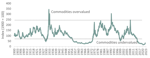
When investing in natural resource equities, the commodity capital cycle is far more important than the broad economic cycle. From this perspective, 2022 is the mirror image of 2008. Our readers will recognize the following two charts. The first chart shows the relationship between the Dow Jones Industries Average and a commodity index going back to 1900. The second chart shows the weighting of energy and materials in the S&P 500. Together these two charts tell a fascinating story.

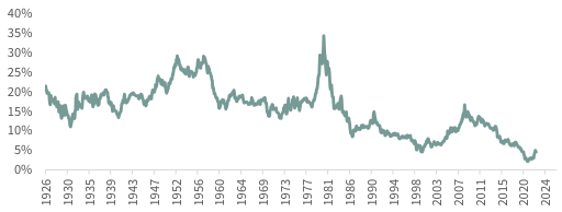
As the top chart clearly shows, commodities go through periods where they become extremely cheap relative to financial assets. At this point, they represent excellent investments and spend years in a bull market. Eventually, commodities become radically overvalued and represent poor investments. The most extreme periods of commodity undervaluation took place in 1929, 1969, 1999 and 2020.

THE FIRST THREE PERIODS WERE EXCELLENT OPPORTUNITIES TO BECOME A NATURAL RESOURCE EQUITY INVESTOR, AND WE STRONGLY BELIEVE THE LAST ONE WILL BE TOO.

It is not a coincidence that periods of commodity undervaluation are good entry points for natural resource investors, nor is it a simple story of mean reversion. Instead, periods of radical commodity undervaluation are related to the natural resource capital spending cycle, and it’s this capital spending cycle that leads to huge outperformance going forward.

A commodity price cycle usually follows a typical path. The industry might enjoy a period of very high energy or metal prices. Given their fixed cost base, the higher commodity prices fall directly to the bottom line resulting in a period of super-normal profits. High returns attract new capital and before long the industry begins a new cycle of exploration and development. Over time, increased spending leads to new supply which eventually outpaces demand growth and ushers in a period of commodity surplus.

Prices fall, causing projects that were underwritten at higher prices to become impaired and written off. Often, another industry or investment strategy falls into favor around this time and investors rush to reallocate capital towards hot new speculative areas, leaving the resource industry even more capital starved. As depletion takes hold, supply falters, demand grows, and inventory gluts eventually get worked off. The stage is set for the next bullish cycle to start.

Investing in natural resource equities when commodities are cheap relative to financial assets is important, not only from a value perspective but also because it almost always corresponds with a bottom in the natural resource capital investment cycle — a cycle that produces years of supply shortages that is fixed only after years of increased spending.

The key insight here is that the commodity capital cycle may or may not correspond with the broader business cycle (i.e., expansion and recession). Heading into the GFC, the two cycles were in near-perfect alignment. Commodity prices were extremely high relative to the stock market in early 2008. Energy and materials made up 20% of the S&P 500 – a 30-year high. Natural resource capital spending had accelerated. Driven by high prices, insatiable Chinese demand, and endless analyst calls for a commodity “super-cycle,” energy and mining capital spending in the S&P 500 surged four-fold between 2000 and 2008 from $80 bn to an all-time high of $330 bn per year.

When the recession arrived, the commodity sector was hit hard. Energy stocks fell by 50% while mining stocks fell 65%, gold stocks fell 25%, and agriculture related equities fell 40%. Natural resource equities rebounded in 2009 and into 2010, but then entered a decade-long bear market. The capital spending surge during the bull market of the middle-2000s ultimately resulted in new production of almost everything: iron ore, coal, copper, shale gas, and oil. The GFC represented a rare alignment of a bearish commodity capital spending cycle and a bearish broader business cycle.

It is no wonder that investors are skeptical of natural resource investments given the experiences of the GFC. However, we think focusing solely on one episode risks missing the point. As it relates to natural resources, the GFC was an anomaly: for most of the past 120 years, the commodity cycle and the business cycle have not been in sync at all. In fact, throughout the twentieth century, resource equities have actually been good investments during most recessions.

To illustrate our point, let’s look closely at the 1930s. The Great Depression was unrivaled in its severity. In the United States, one person out of every four in the labor force was without work. Industrial production fell 50% from peak to trough and took a full decade to regain its pre-crash high. Wholesale prices collapsed by 30%, and the stock market fell 86% from its 1929 high. Equities did not regain their pre-crash 1929 highs until 1954. Even factoring in dividends, anyone who invested in 1929 only broke even in 1946.

The financial system became severely impaired; the situation became so dire that in 1933, FDR announced a “bank holiday,” effectively closing the US financial system for seven days. Between 1930 and 1932, the United States saw 7,000 banks fail.

Given their economic sensitivity, it is reasonable to think that commodities and natural resource equities must have fared terribly during the Great Depression. Surprisingly, natural resource investments did not collapse during the Great Depression; they turned out to one of the best performing asset classes. A simple equity portfolio made of equal positions in gold miners, oil producers, base metals miners, and agriculture companies made just before the stock market collapse in September 1929 more than doubled a decade later.

By comparison, at the end of the period in 1937 the total return of the S&P 500 was still down nearly 50%. By 1946, when an investment in the S&P 500 finally reached its pre-crash levels, the same natural resource equity portfolio had tripled.

HOW COULD A PORTFOLIO OF ECONOMICALLY SENSITIVE STOCKS LEAD THE MARKET DURING THE WORST ECONOMIC COLLAPSE IN HISTORY? THE ANSWER IS THE NATURAL RESOURCE CAPITAL CYCLE.

Commodity prices fell throughout the 1920s and by 1929, had become radically undervalued relative to financial assets. Just as important, low commodity prices starved the industry of capital throughout the decade.

The Roaring Twenties bypassed the natural resource sector entirely, with many investors dismissing producers as no longer relevant in an economy being driven by things like radio and advertising. Instead, traders flocked to growth stocks, notably utilities, automobile manufacturers, and radio companies. Radio Corporation of America (RCA) was the “tech” stock of the day. By 1929, the oil industry was trading at a price to book valuation of only half the broad market. The energy and materials weighting in the S&P 500 fell steadily throughout the 1920s as investors diverted capital to higher returning (and more speculative) sectors.

In many ways the natural resource bear market of the 1920s was predictable in that it was driven by the capital cycle boom of the 1910s. From 1900 to 1910, oil prices surged more than threefold. Oil producers enjoyed a period of super-normal profits and capital rushed in and a full-blown oil exploration boom took place. Huge new discoveries were made in Texas, Oklahoma, California, Colorado, and Kansas. By 1920, crude oil prices peaked at $3.07 per barrel – up five-fold in 20 years.

Between 1917 and 1927, US crude production surged by 400%, or almost 15% per year. The market swung into massive surplus, and inventories swelled from 130 mm bbl to over 550 mm bbl – this inventory figure was the highest level ever recorded, according to the US Energy Information Agency (EIA), excluding today’s Strategic Petroleum Reserve (SPR).

Surging inventories depressed oil prices throughout the 1920s and by 1928 crude had fallen by 70% from $3.07 to $1.17 per barrel. Profitability in the energy industry collapsed, and investor capital, chasing speculative returns elsewhere, fled the industry.

When the Great Depression hit, oil demand was initially impacted, but it quickly recovered. Capital-starved supply on the other hand could not keep up. From 1929 to 1934, US crude production declined — the first time US production had ever declined over a five-year rolling period. US production would not undergo such a sustained decline again until the late 1970s when conventional supply entered terminal decline. Even by the late 1930s, annual production growth was only averaging half the level of the 1920s.

Crude inventories actually peaked in September 1929, right as the Great Depression started, and spent the next decade falling sharply, suggesting a persistent structural deficit. Given these dynamics, oil equities were able to rally during the darkest days of the 1930s. Between 1929 and 1937, oil stocks returned 30% compared with the S&P 500 that was still down nearly 50%. Between 1929 and 1947, when the S&P 500 was finally breaking even, oil stocks had nearly tripled on a total return basis.

Unfortunately, we do not have the same level of detail on metals inventories during the 1930s, however we can still make some important qualitative observations. Just like oil stocks, base metals stocks were extremely out of favor throughout the 1920s and spent the decade drifting lower as investors diverted their capital elsewhere. Throughout the 1910s, demand for every metal skyrocketed driven by World War I. Prices surged and companies increased production.

When hostilities ended in 1918, the world found itself with far too much mine production and scrap material and prices collapsed. Throughout the 1920s, the price of copper fell steadily by 85% from 60 cents to 8 cents per pound. Mining companies, who made their investment decisions in a much higher price environment, found themselves struggling and several were forced to write off assets and declare bankruptcy. By the beginning of the Great Depression, the mining industry had been starved for capital for an entire decade and hardly any new capacity had been sanctioned.

As a result, even the famously economically sensitive copper was able to do well during the Great Depression. Mining companies saw their product price increase modestly throughout the 1930s given tight mine supply. At the same time, the collapse in wholesale prices drove costs lower. Mining stocks were one of the only sectors that experienced improved profitability throughout the turmoil of the 1930s and investors responded favorably. Between 1929 and 1937, mining stocks returned 30% and by 1947 they had doubled.

Gold stocks were by far the best performers throughout the Great Depression. Britain’s decision to abandon the gold standard and devalue the pound in 1931, coupled with the partial collapse of the banking industry in the United States, resulted in huge amounts of gold leaving the US Treasury. By 1934, the United States made the decision to devalue the dollar by changing its convertibility into gold from $20.67 per ounce to $35. Gold mining stocks saw their revenues jump 70% at the same time as their costs collapsed. Profitability soared as did share prices. Between 1929 and 1937, gold stocks increased five-fold, representing compounded growth of 17% per annum.

Although it may sound extremely counter-intuitive given how economically sensitive they are thought to be, natural resource stocks were actually one of the only places to hide (and even thrive) during the Great Depression. The reason was the commodity capital spending cycle and the clue was that commodities were cheap relative to the broad market.

For those fearing a recession, what happened to commodity related equities in the Great Depression is a great example of what might happen today if a severe recession gripped the global economy. The radical undervaluation of commodities and commodity related equities is greater now than it was back in 1929, and the level of capital starvation is just as great. History tells us that commodities could again be an excellent place to seek high returns, even if the 2020s experience a period of economic turmoil as severe as the Great Depression — a scenario we consider unlikely.

In 1969 and 1999, commodities reached radically undervalued levels once again. In both cases, commodity prices had spent at least a decade falling and companies again became capital starved. It’s no surprise these were excellent times to become a natural resource equity investor. Between 1970 and 1980, the same equal weighted portfolio of miners, oil companies, gold stocks, and agriculture companies advanced 500% while the S&P 500 was up 170% — barely keeping up with inflation. Two recessions that decade (one severe) had very little impact on commodities and natural resource equities did extremely well.

Between 1999 and the GFC in 2008, the same portfolio would have returned nearly 400% compared with only 20% for the S&P 500. The dot-com market collapse of 2000 and the recession of 2001 did not stop natural resource equities from posting their strongest decade ever.

In this context, the GFC was indeed a unique episode in which the commodity capital cycle and the business cycle were in sync. After several years of strong performance capital had rushed in and new projects abound. As a result, prices fell sharply during the GFC, recovered somewhat, and then entered a 10-year structural bear market.

Today conditions couldn’t be more different than those preceding the GFC. Commodities and natural resource equities have never been cheaper and more out of favor relative to financial assets. In 2020, energy and materials made up less than 2% of the S&P 500 compared with 20% in 2008. Because of the 2010-2020 commodity bear market, capital spending for almost all extractive industries has been severely curtailed.

For example, in the energy industries, capital spending in the S&P 500 has fallen from $320 bn per year to less than $100 bn today and, as you will read in the “Incredible Shrinking Super Majors,” what capital remains is not being spent efficiently. Given this backdrop, which far exceeds the extremes of 1929 (at least concerning valuation), even a severe economic contraction that rivaled what happened back in the 1930s should still offer excellent returns in commodity, and commodity related investments.

In the meetings we mentioned earlier, we learned that institutional investors who run 60/40 portfolios are extremely worried about adding a natural resource related investment to their standard mix. Historically, adding natural resource investments at the bottom of commodity capital and valuation cycles (where we are right now) would have dramatically improved future performance. During the 1929-1939 period, for example, a classic 60/40 portfolio would have returned 0%, with large gains in the bond portfolio offsetting large losses in equities.

Reallocating 20% from the broad equity bucket to the natural resource equity portfolio discussed above would have reduced risk and added return. Instead of being flat over the decade, a 40/40/20 portfolio (40% equities, 40% bonds, 20% natural resource equities) would have returned 3.4% per year all while reducing volatility from 23% to 20%. During the 1970s, the 60/40 portfolio returned 8.4% per annum while a 40/40/20 portfolio returned 10.3% while maintaining risk at 10.4%. From 1999 to 2008, the 60/40 portfolio returned 3.7% per annum compared with the 40/40/20 that returned 7.0% while maintaining risk at 9.8%.

Investors find themselves confronted with a market unlike any they have experienced: inflation is high, growth is difficult to come by, and raw materials are in short supply after a decade of capital starvation. Even under the most strained deflationary and inflationary periods experienced in United States history, commodities and their related equites produced large positive nominal and real returns. Unfortunately, most investors remain woefully under-allocated to this important sector — ironic given commodity related equities may be the only thing safeguarding capital in the years to come.

The Incredible Shrinking Supermajors Part III

“Are you embarrassed as an American company that your production is going up while the European counterparts are going down…. Would you commit to matching your European counterparts to reducing the production of oil?”

Questions asked of the CEOs of Chevron (CVX) and Exxon (XOM) by Ro Kanna (D), Member House of Representatives and Chairman of the Subcommittee on the Environment during a October 28, 2021 congressional hearing.

“At a time of record profits, Big Oil is refusing to increase production to provide the American people some much needed relief at the gas pump.”

Frank Pallone (D), Chairman of the House Energy and Commerce Committee during an April 6, 2022 Congressional Hearing.

In previous letters we discussed the plight of the energy supermajors and how significant reductions to their upstream capital spending would translate into shrinking hydrocarbon production. Under severe pressure from ESG forces (notably activist shareholders and belligerent governments), the supermajors have indeed significantly slashed upstream capital spending with serious impacts to oil and natural gas production.

First, Exxon was targeted by an activist group calling on it to significantly reduce upstream spending. Despite owning just 0.02% of Exxon’s stock, Engine No. 1 demanded and received 25% of Exxon’s board seats.

Next, in response to civil charges brought forward by seven environmental activists, a Netherlands court ruled that Royal Dutch Shell, Europe’s largest oil company, must accelerate its effort to reduce carbon emissions 45% by 2030. Making matters worse, Shell was then attacked by activist shareholder Third Point Management, demanding they break into two companies. The first company would hold the traditional oil and gas assets which would be starved for capital. Spending would be redirected into the second company, holding all the renewable investments.

Third, following its success in gaining access to Exxon’s board, Engine No. 1 sat down with Chevron’s senior management. Although we do not know what was discussed, Chevron later stated that they were more committed than ever to reducing their carbon emissions and were seeking a new director with “environmental expertise.” Clearly Engine No. 1’s success with Exxon made a serious impression on Chevron’s management. Only four months after meeting with Engine No. 1, Chevron announced a $3 bn bio-diesel investment — an acquisition we will discuss in a minute.

Finally, the CEOs of Exxon, Chevron, Shell (SHEL), and BP were dragged before the Congressional House Oversight Committee and castigated not only for misleading the public about climate change, but also for not doing more to restrict oil and gas spending.

Six months later, with gasoline prices surging, the supermajors were again summoned to yet another congressional hearing. This time, they were asked why they were not increasing spending in their traditional oil and gas business.

Recently, President Biden wrote a letter to seven of the largest oil companies urging them to produce more crude and refined products. His letter called on major oil companies with large refining capacity to take immediate actions to ramp supply. “Historically high” prices at the pump are not “acceptable,” he warned before ending with a threat: “I am prepared to use all tools at my disposal, as appropriate, to address barriers to providing Americans affordable, secure energy supply.”

BEING A SUPERMAJOR IS GETTING MORE AND MORE DIFFICULT: CLIMATE CHANGE, ASSAULTS BY ACTIVISTS’ SHAREHOLDERS AND ANGRY GOVERNMENTS, AND PROBLEMS IN RUSSIA (WHERE THE SUPERMAJORS HAVE ALL MADE SIGNIFICANT INVESTMENTS). THE NET RESULT OF THESE STRESSES TODAY IS OBVIOUS: THEY ARE SHRINKING.

The downward pressure on upstream capital spending, so desired by the ESG crowd, is having the desired results. Even though oil prices averaged over $100 per barrel and gas spiked to $300 per barrel of oil equivalent, spending is only now starting to increase. We have commented repeatedly how this constriction and redirection of capital would eventually produce large consequences and unfortunately, they are now being felt with a vengeance.

Q2 upstream capital spending for our five supermajors (Exxon, Chevron, Shell, Total, and BP) rose a significant 15% sequentially and 30% year-over-year. It is important to note however that 70% of the $1.7 bn sequential increase came from one company — Shell.

Over the last four years, Shell led the supermajors in reducing upstream capital spending (almost 50%) with predictable results. Total hydrocarbon production fell 35% since 2019 — the worst in the group. Excluding Shell’s material upstream capital spending increase, the four remaining companies increased spending only 5% sequentially and 18% year-over-year.

Capital spending for our supermajors remains 30% below the 2019 level (even with Shell’s big increase) and an incredible 60% below the 2010-2016 average.

In response to years of inadequate upstream spending, the supermajors’ production of oil and natural gas continues to fall. Second quarter liquids production fell 2% sequentially and 4% year-over-year. Natural gas production fell 4% sequentially, and 3% year-over-year.

Since the beginning of 2019, liquids production is down 12% and natural gas production is down 16%, while spending is down 20%. Because of restricted upstream capital spending, the supermajors are 14% smaller on a BOE basis than just three years ago – very much in line with what we predicted in our 2021Q2 essay.

ESG pressures have forced the supermajors to shrink their upstream businesses. Other consequences are now emerging as well. Large sums are being redirected away from the traditional upstream businesses, which sport extremely high energy efficiency, into renewables which are much less efficient.

Nothing demonstrates this better than what Chevron did back in February. Rattled by Engine No. 1’s Exxon success, Chevron committed to invest $10 bn to reduce its carbon emissions through 2028 and be completely carbon neutral by 2050. As a first step, Chevron announced the acquisition of Renewable Energy Group, an Iowa based producer of biodiesel and renewable diesel, for $3 bn.

Biodiesel is a renewable fuel that is manufactured from vegetable oils, animal fats, and recycled restaurant grease. Although “advanced biodiesel” and “renewable diesel” might earn Chevron some ESG bone fides, we should stress that biodiesel will do little to reduce the overall level of CO2 in the atmosphere. Furthermore, the energy efficiency of biodiesel is so much worse than traditional hydrocarbons that both society and the environment are ultimately left worse off.

Consider this: Chevron spent $3 bn to acquire Renewable Energy Group. The acquisition will produce 32,000 b/d or 11.5 mm barrels per year of biodiesel. Assuming the assets last 20 years, Chevron will produce 230 mm barrels of biodiesel over the coming two decades. How does this compare to a traditional upstream investment? Assuming Chevron instead invested this $3 bn in their prime Permian basin acreage, and that a Permian barrel can be drilled, completed, and produced for $12, a comparable investment would produce 250 mm barrels of oil equivalent – 9% more than the biodiesel.

These figures do not tell the whole story. With the Permian investment, 80% (or 200 mm bbl) are produced within the first four years. In other words, it will take the biodiesel plant 17 years to produce what the conventional oil and gas investment produces in four.

Furthermore, manufacturing biodiesel is incredibly energy intensive. The hydrocracking process used to turn waste fats and oils into biodiesel requires a huge amount of energy as does growing, harvesting, and processing feedstock crops (i.e., soybeans, dates, sunflowers, seeds, etc).

We calculate the total energy returned on energy invested (EROEI) for manufacturing biofuels is only 2.5 or 3:1. By comparison, the production of diesel from crude oil is extremely energy efficient. For every unit of energy used to drill, produce, transport, and refine a barrel of oil into diesel, 30 units of energy are released when it is consumed – diesel has an EROEI of 30:1.

With 6.1 GJ contained in every barrel of oil (or diesel), were Chevron to invest $3 bn in the Permian, it would produce 1.2 bn GJ of energy in just the first four years. Assuming a 30:1 EROEI, Chevron would expend only 40 mm GJ of energy in the process, leaving 1.16 bn GJ of net usable energy in the first four years.

By comparison, Chevron’s $3 bn investment in Renewable Fuels would yield spectacularly less. In the first four years, Chevron’s biodiesel investment will produce 50 mm barrels of biodiesel with gross contained energy of 300 mm GJ – already 75% less than the Permian. However, the EROEI is so poor, 100 mm GJ will be consumed just to produce this already diminished output. Therefore, Chevron’s biodiesel operation will produce only 200 mm GJ of net usable energy over the first four years, compared with 1.16 bn GJ in the Permian — a reduction of nearly 85%.

Over its full 20-year life, Chevron’s biodiesel investment will eventually produce 230 mm barrels, but again the low EROEI will consume 35-40% of the embedded energy. We estimate that over 20 years, the biodiesel operation will only produce 925 mm GJ of net usable energy – 40% less than the 1.5 bn net GJ produced from a comparable investment in the Permian.

A conventional hydrocarbon investment will generate more usable net energy and will deliver it much more quickly. The world is currently in the midst of an acute energy crisis. Diversifying out of hydrocarbons towards things like biodiesel will only make the current crisis much worse.

THE DEEPER ONE INVESTIGATES CHEVRON’S BIODIESEL ACQUISITION THE WORSE IT GETS. THUS FAR WE HAVE DISCUSSED ECONOMICS AND ENERGY INTENSITY, BUT EVEN FROM A CO2 PERSPECTIVE, BIODIESEL MAKES LITTLE SENSE.

Because of its extremely low energy efficiency, CO2 produced from manufactured biodiesel is at best on par with diesel refined from crude oil and at worst is much greater. We calculate that each barrel of diesel sourced from conventional hydrocarbons releases 460 kg of CO2 – 440 kg released during the combustion itself and 20 kg emitted during the drilling, transporting, and refining of the crude oil.

A barrel of biodiesel will still emit the same 440 kg of CO2 during combustion, but instead of emitting 20 kg during its manufacture it will now generate 230 kg due to the low EROEI. In total a barrel of biodiesel will release 670 kg of CO2 compared with 460 kg for conventional diesel – an increase of 45%. Offsetting this inefficiency is the fact that the biodiesel feedstock will capture and sequester carbon as the plant grows due to photosynthesis. The question becomes how much carbon the feedstock for a barrel of biodiesel can sequester.

This critical metric depends on the feedstock (i.e., corn, soybeans, etc.), the farming techniques (i.e., fertilizer application, responsible farming, etc.), and whether the feedstock is grown for diesel or waste products are used. The key issue is whether ultimately the feedstock can sequester at least 210 kg of CO2 per barrel of biodiesel to offset its inherent energy inefficiency.

As you can imagine, the analysis becomes fiendishly difficult, but there is a growing consensus that under the best scenarios, biodiesel’s carbon intensity is on par with diesel and at worst it is much greater.

Chevron made a $3 bn investment to deflect potential activist harassment, like what happened to Exxon and Shell. Unfortunately, we believe this investment made little operational sense. It is terribly energy inefficient on both a short- and long-term basis. Even stretching the energy recovery period over 20 years, Chevron’s biodiesel business will produce 40% less energy than a comparable investment in the Permian. Next, from a CO2 output standpoint, amount of CO2 produced from a manufactured barrel of biodiesel is at best even and at worst 45% greater than the CO2 produced from crude-oil based diesel.

The supermajors are pouring billion and billions into another area with inferior energetics: offshore wind. In just the last year BP, Shell, and Total have committed to a massive offshore wind build-out off the coast of New York and New Jersey. BP announced three huge offshore wind projects off the coast of Massachusetts and Long Island. The estimated installed capacity for all three projects (Beacon, Empire Wind 1 and Empire Wind 2) totals 3,300 megawatts.

BP will own 50% in all three projects. Shell has announced its 50% interest in the newly awarded Atlantic Shores Offshore Wind Bite project off the coast of New Jersey with an installed capacity of 925 megawatts. Total announced its 100% interest in the Attentive Energy project off the coast of New Jersey with estimated capacity of almost 1,000 megawatts.

Rising steel, concrete, and copper prices over the last three years have caused the capital cost on these projects to soar. In 2015, we calculated that it cost $3.50 to $4.00 per watt to build and install offshore wind capacity. Since then steel, cement, and copper prices have all risen more than 75%, driving capital costs to as much as $5 to $6 per watt.

Using $5.50 per watt as a base, the wind projects just discussed will now cost Shell, BP, and Total a combined $17 bn for 3,100 megawatts net to them. BP will be on the hook for $9 bn to build 1,650 megawatts net to them. Shell will invest $2.6 bn to build 465 megawatts net to them and Total will need to invest $5.5 bn to build out their 1,000 megawatts of power.

Just like Chevron’s biodiesel acquisition, these massive wind investments will make the current energy crisis much worse. Windfarms, much like biodiesel, have a vastly inferior energy efficiency compared with traditional hydrocarbons. On an “un-buffered” basis — that is, without any storage backup — the best offshore windfarm produces in an EROEI of 10-15:1. “Buffering” the wind farm with battery storage (desperately needed, but so far barely implemented), drops the EROEI to between 5-10:1, compared with 30:1 for traditional hydrocarbons.

Clearly offshore wind compares unfavorably with offshore oil and gas. How unfavorably? Assuming that an un-buffered offshore wind farm will be operating with a 37% load factor for 20 years, the supermajor’s $17 bn investment will generate 10 mm mwh per year or 200 mm mwh over two decades. This equates to 36 mm GJelec per year or 720 mm GJelec total.

If our supermajors had instead taken this $17 bn and invested in a traditional hydrocarbon project (say a large offshore development), the results would be much different. Assuming total finding and development costs of $25 per boe, they would have produced some combination of 680 mm bbl of oil and 4.8 tcf of natural gas.

If this natural gas was piped onshore and burned in a combined-cycle natural gas plant sporting a “heat-rate” of 60%, the investment would ultimately produce 122 mm GJelec per year or 2.45 bn GJelec over its 20-year life.

Again, the difference in net energy produced between a renewable energy project and a traditional hydrocarbon project is huge. The offshore wind farms will wind up producing 70% less power than a similar investment made in offshore hydrocarbon projects over their full useful lives.

Back in 2020, Wood Mackenzie, the energy consultant, estimated that well over $200 bn would be invested in offshore wind farms in the next several years. They believed that the oil and gas industry, which at the time had little in the way of offshore wind farm exposure, had the potential to become a huge participant. For example, Equinor (EQNR), the Norwegian oil and gas company, has stated that they plan to invest in as much as 6,000 megawatts of offshore generating capacity in the next six years and by 2035 to have 16,000 megawatts.

And please note that Equinor has already aggressively committed itself to entering this market—Equinor is the 50% partner with BP in the Beacon, Empire Wind 1, and Empire Wind 2 projects. We estimate Equinor will have to invest up to $100 bn to build-out these 16,000 megawatts of capacity. Spending levels of this magnitude will prevent Equinor from investing in its traditional upstream business. For example, over the last 10 years Equinor has spent approximately $140 in upstream capital spending, so you are talking about a huge diversion of capital amounts (up to 70%) that will now be invested in energy projects that will produce 70% less energy.

As the examples above clearly show, the supermajors have already begun to divert significant amounts of capital away from their traditional upstream business. In the case of Chevron’s investment in renewable biodiesel, the energy ultimately produced by this investment will fall by almost 80% and the amount of CO2 produced at best will be the same and at worse be 45% higher. In the case of offshore wind, the investments needed are huge, but the drops in actual energy produced are huge as well—approximately 70%.

The cutbacks in upstream capital spending by the supermajors has already impacted traditional upstream production—the supermajors are shrinking very much in line with the projection we made in our first essay on the “Incredibly Shrinking Supermajors” back in the Q2 2021. Now, it looks like these supermajors, because of intense ESG pressure, are diverting huge amounts of capital away from their traditional high EROEI oil and gas businesses into ventures with energy efficiencies that are 80% lower. The energy crisis we are in now will only be made worse by what the supermajors are doing.

In our next installment of this series on the incredibly shrinking supermajors, we will discuss BP’s massive new investment in the Asian Renewable Energy Hub (AREH). Estimated capital cost of this project could approach $25 bn ($10 bn net to BP). We will discuss its terrible energy efficiency, another example of how the supermajors are destroying themselves in an attempt to placate the hostile ESG pressures now pushing in on all sides. We believe BP’s investment in the AREH project will be a huge mistake.

In the case of BP’s Australian hydrogen project, you are combining the unconventional production of electricity ((wind)) with the production of hydrogen, another highly unconventional energy source. Combining the incredibly low energy efficiency of windfarms with hydrogen manufacturing is a guaranteed recipe for failure. There is a saying in the oil and gas business that you cannot combine two unconventional elements in a major project. We believe BP’s investment in the AREH project attempt just that – and will ultimately produce extremely low returns.

High Energy Cost Hurts Wind & Solar

Our 4Q2021 letter was entitled “The Distortions of Cheap Energy.” In our lead essay, we explained how extremely low energy prices throughout the 2010s distorted the cost of several energy transition technologies, notably wind, solar and lithium-ion batteries. Between 2010 and 2020, the cost of each of these technologies fell by more than 70%. Most investors believe the reduction was driven by a variation of Moore’s Law known as the “learning curve.”

According to this model, the industry would get ever more cost efficient the more units were installed.

After having studied the wind and solar industries for years, we had a radically different view. Wind and solar are extremely energy intensive forms of power. The ubiquitous (albeit now modest) 1.5 MW GE wind turbine contains 40 tonnes of steel and 600 tonnes of concrete in the foundation alone. The tower adds another 150 tonnes of steel while the generator requires 9 tonnes of copper. All these materials require huge amounts of energy to mine, process and refine. Between 2010 and 2020, the cost of every form of energy – whether it be oil, natural gas, coal or uranium – fell by 90% from peak to trough.

It stands to reason that much of the reduction in the cost of renewables can be attributed to lower energy prices. Furthermore, renewables are very capital intensive. Over the past decade, we have experienced the lowest cost of capital in human history. Again, it is likely this too contributed to falling renewable energy cost. As simple as these insights were, no one else seemed to be talking about them. Instead, the industry and Wall Street analysts were convinced that renewable energy costs would continue to move ever lower – oftentimes contradicting the very laws of physics.

WE BUILT A RENEWABLE ENERGY COST MODEL THAT EXPLICITLY INCORPORATED ENERGY AND CAPITAL COSTS. WE CONCLUDED THESE TWO FACTORS ALONE WERE RESPONSIBLE FOR MOST OF THE DRAMATIC COST REDUCTION IN WIND AND SOLAR COSTS BETWEEN 2010 AND 2020. AS THE ERA OF CHEAP ENERGY AND CHEAPER CAPITAL CAME TO AN END, WE ARGUED THE COSTS OF RENEWABLE ENERGY WOULD STOP DECLINING AND MIGHT ACTUALLY BEGIN TO RISE.

Since then, our models appear to have been proven correct. According to Bloomberg New Energy Finance, the cost of wind rose by 10% between the first quarters of 2021 and 2022 while solar rose 12% and lithium-ion batteries rose 15%. The culprit in all cases was a combination of rising material prices (themselves a function of higher energy costs) and higher capital costs. Earlier this year, LG announced it would shutter its solar panel division amid higher input costs. Our models suggest this is merely the first company to announce such a move.

While we have mainly focused our analysis on costs, there is now a more acute problem with renewables. The world finds itself in the midst of an immediate energy crisis. After years of underinvestment, the cost of every energy source has gone from record lows to record highs (in real terms) in only two years. The past ten years of abundant reliable energy now seem to be over. If energy continues to be scarce and dear, we simply cannot afford the high energy cost of renewable power.

In our past letters, we have detailed the concept of energy return on energy invested, or EROEI. Every source of useable energy consumes some of that energy in its own generation. The ratio energy-out to energy-in is known as the EROEI. For example, hydrocarbons generate 30 units of usable energy for every unit of energy consumed while the best unbuffered windmill might generate 10 units of energy for every unit of energy consumed. In other words, wind power is 65% less efficient than hydrocarbons on an EROEI basis.

However, looking at EROEI alone does fully capture the current situation. In the case of hydrocarbons, nearly all the usable energy is generated within the first five years. We can naively assume that an oil or gas well will generate six times the energy expended for five years before falling to basically zero (6:1 for 5 years gets you 30:1). Every unit of energy expended in such a system will have an immediate positive impact on total energy availability effective immediately.

Renewables on the other hand are entirely different. Our ideal windmill that enjoys and EROEI of 10:1 will produce power (mostly) evenly over its 25-year life. Therefore, in any given year of operation, the windmill will only return 40% of the energy necessary for its manufacture and installation.

In a world of abundant energy, society can energetically afford to invest in windmills and solar farms. However, when faced with an immediate energy crisis like we have today, every incremental unit of renewable energy will only make the problem worse.

There is still today a widely held belief that rising energy costs will make renewable power more competitive. This naïve view neglects just how energy intensive renewable power truly is. Policy makers would be advised to understand these limitations before enacting major renewable subsidies that will only make the current energy shortage that much worse. Europe’s $1 trilllion investment in wind and solar has produced the worst energy crisis in decades.

Given the recent passage of the Biden administration’s “Inflation Reduction Act,” with its billions in subsidies for various low EROEI renewable projects, we believe the US is now travelling down the same road as Europe.

Natural Resource market Commentary – 2Q22

After putting in their best performance in over 30 years, commodity prices experienced a broad-based pullback in Q2. Hawkish language from the Federal Reserve, continued COVID and property development issues in China, and fears of a global economic slowdown put downward pressure on most commodity prices. The only commodities bucking the downward trend and showing strength were oil, European and Asian natural gas, and global thermal coal.

Given its high exposure to energy prices, the Goldman Sachs (GS) commodity index rose 2% during the quarter, whereas the Rogers commodity index, which has more agricultural and metals exposure, fell 2%. Commodity related equities were weak during the quarter. However, since January 1st, natural resource equities have significantly outperformed the general stock market. After surging 29% in Q1, the S&P North American Natural Resource stock index, which has significant exposure to large capitalization energy, fell 10.6%. For the year it’s up 15.5%.

The S&P Global Natural Resource Index, which has much higher agricultural and metals equity exposure, gave back its 16% gain experienced in Q1. In comparison, the overall market, as measured by the S&P 500 stock index, fell over16% during Q2, and is now down 20% for the year.

Oil

Even with the announcement on March 31st that the US government, in coordination with Japanese and European governments, would release almost 1.5 mm b/d of oil from their strategic petroleum reserves for the next six months, oil prices continued to move higher. During the second quarter, US oil prices, as measured by the West Texas Intermediate benchmark, rose over 5%, whereas Brent prices rose almost 8%.

Even with fears of Chinese economic slowdowns and demand destruction, the global oil market continues to get tighter and tighter—a tightness that is being masked by the SPR releases and is being ignored by almost everyone. In their latest “Oil Market Report,” the IEA made no mention of how SPR releases were behind the slight inventory build experienced over the last three months. Global oil inventories are steeply declining after stripping out the SPR releases—a point the IEA refuses to acknowledge.

Plunging inventories, disappointing production growth from both the US shales and non-OPEC counties, and demand strength that continues to confound all the oil bears are covered in the oil section of this letter. We also revisit the issue of Saudi Arabia’s pumping capability. With more energy analysts now publicly admitting that that OPEC’s pumping capability may be overstated and given that oil markets will need every barrel of stated pumping capability in order to meet market demand in Q4, it is of utmost importance to know whether the Saudis can indeed pump the 12 mm b/d they claim.

In this letter, we update our Saudi pumping capability study given that three years have passed since our original thoughts.

Global Demand is running significantly higher than consensus admits, supply continues to disappoint, and we believe pumping capability will reach its limit in Q4 – a first in 160 years of oil market history.

Natural Gas

Natural gas prices on a global basis were mixed. US prices slipped 4%, whereas European natural gas continued to surge, rising an additional 20%. Asian prices rose 3%. The divergence of North American gas prices and global natural gas prices continues in the extreme. Today, European natural gas prices have surpassed $60 per mmbtu ($360 per barrel in oil terms) and Asian prices are $43 per mmbtu ($260 per barrel). In contrast, US natural gas prices are at $8.20 per mmbtu.

We still firmly believe that US and global gas prices will begin to converge in the next six months — a subject we covered at great depth in our last letter — even with the fire at the Freeport LNG export facility which took place on June 8th. That fire took offline 2 bcf per day of LNG export capacity for at least six months. However, because of hot weather, we continue to draw US natural gas inventory levels down faster than normal, a subject that almost no analyst is commenting on.

Read the natural gas section of this letter where we talk about the intensifying natural gas crisis in Europe and the increasing bullish supply demand issues that continue to develop here in the United States.

Coal

Global coal prices continued to strongly advance in Q2, as the global natural gas crisis continued to spill over and affect global thermal coal markets. Australian thermal coal prices advanced 50% and Richard’s Bays (South African exported thermal coal) prices advanced 35%. Here in the US, Illinois Basin high sulfur thermal coal advanced 30% and Central Appalachian thermal prices rose 60%. For the year, thermal coal prices have been the best performing asset class, only matched by European natural gas prices.

Year-to-date Illinois Basin prices are up 180%, Richard’s Bay prices are up 150%, and Australian Thermal prices are up 130%. Although we are long-term believers that coal will ultimately be displaced by nuclear power generation, we argue that the global natural gas crisis, which we believe still has years left to play out, will continue to put upside pressure on coal prices. Several leading coal equities now trade at price-to-earning ratios of 3 or less.

As some of you might remember, we were huge investors in the global coal market when I ran the Chilton Global Natural Resource fund and we know global coat markets extremely well. The bull market in coal today is being driven by massive policy errors from the last decade—namely the huge investments made in the global renewable power business. In the next letter, we will write extensively on global coal market fundamentals, and how coal, the fossil fuel that everyone loves to hate, could very well be the biggest beneficiary of these policy errors.

Uranium

After peaking at almost $60 per pound in the mid-March, spot uranium prices pulled back to $48 per pound by the end of Q2. Long-term contract prices, however, continue to edge higher. Starting at $49 per pound at the end of Q1, long-term contract prices finished Q2 at $52 per pound.

The positive shift toward the adoption of nuclear power generation continued strongly in Q2. On July 6, the European Parliament backed the previous adopted rules that labelled investments in nuclear power plants as climate-friendly and threw out an attempt to block the law by various climate-activist groups. By including nuclear power in the taxonomy, the European Union has confirmed its commitment to expand nuclear power generation as a climate friendly option—an extremely positive development for the reemergence of European nuclear power.

In December of last year, the Netherlands announced plans to construct two new nuclear power plants and France has announced plans to build up to 14 new-generation reactors plus a fleet of smaller “modular” reactors as the country seeks to cut its CO2 output and its reliance on Russian energy.

In July, the Japanese government announced that four more nuclear reactors will be restarted in order to avert a power crunch this winter. A total of five reactors have now been restarted. With the addition of these four, Japan has now brought back almost 20% of the 50 reactors that were operating before Fukushima.

Please turn to the uranium section of this letter where we discuss all that has taken place in the last quarter, including the emerging importance of small modular reactors. We remain extremely bullish and have used the weakness in both the uranium spot market and in uranium related equities as an opportunity to increase our exposure and we recommend that investors do the same.

Agriculture

After wheat made all-time highs in Q1 and soybeans and corn just missed making all-time highs, grain prices pulled back in Q1. Continued talk of good growing conditions here in the United States and the potential for ending Russia’s blockade of Ukraine’s grain exports have put downward pressure on grain prices. Wheat prices pulled back the most in Q2, falling 13%. Fertilizer prices, after surging in Q1 also pulled back in Q2.

Nitrogen prices fell 40%, phosphate prices fell 15%, and potash prices fell 10%. We believe we are in a decadelong agricultural crisis that will take many unpredicted twists and turns and argue that all agricultural related equities are still excellent investments. We continue to prefer global fertilizer equities. Not only are fertilizer fundamentals excellent, but the stocks have never been cheaper. Industry leader Nutrien (NTR, the combination of Potash Corp. of Saskatchewan and Agrium) now trades for less than five times earnings.

At the last fertilizer peak, back in 2008, Potash Corp. of Saskatchewan traded for almost 20 times earnings. Both grain and fertilizer prices are in long-term structural bull markets and the stocks represent tremendous value.

Base Metals and Copper

Almost all base metals experienced serious pullbacks in Q2. Aluminum fell 35%, while nickel and zinc fell over 25%. Copper held up slightly better, falling 22% in price. Copper and base metals related equities were also very weak. Copper equities (as measured by the COPX ETF), and base metals equities (as measured by the XBM ETF), both fell 32% — twice as much as the general market. Copper continues to be our favorite base metal.

In July 2016, we wrote an essay on the huge impact of renewables on copper demand going forward. We estimated that the build out of renewable power would cause drive copper demand much higher this decade. At the time, copper sat at $2.50 per pound and investors were universally bearish. Everyone believed demand would weaken and mine supply would continue to grow. No one understood that copper was about to become the green metal and that copper mine supply would disappoint.

It has taken six years, but the massive structural deficit has now become apparent to most industry analysts. As proof, we recommend a look at S&P Global’s recently published whitepaper entitled “The Future of Copper: Will the looming supply gap short-circuit the energy transition.”

In the copper section of this letter, we talk about current supply-demand conditions in today’s market. We will also discuss the S&P Global paper which comes to the same conclusion we did back in 2016. A huge structural gap between demand and supply has emerged, which can only be closed by much higher prices.

Copper and its related equities have experienced large price pullbacks in the last three months. The price of copper made an all-time high of almost $5 per pound in the first week of March and has since pulled back 35%, reaching a low of $3.20. Copper related equities have pulled back similar amounts. Given our bullish outlook, we believe the severe pullback in price in both copper and copper related equities has presented investors with a great buying opportunity.

Gold

After showing strength in Q1, precious metals prices reversed course and fell sharply in Q2. Gold fell 7% and silver fell 19%. Platinum fell 9% and palladium fell 15%.

Precious metals related equities exhibited pronounced price weakness as well. Gold and silver equities, (as measured by the GDX ETF and the SIL ETF), both fell almost 29%. Rising short-term interest rates pushed down precious metals prices. The Fed raised the Fed Funds rate by 50 bps in the beginning of May and an additional 75 bps in June.

We’ve discussed how the rising short-term rates could put downward pressure on gold prices. The precious metals section of this letter explores how the underlying fundamentals in precious metals markets have deteriorated during the quarter, as well as how western physical buyers have switched being sellers once again. Even with the pullback in the gold price, the positioning of traders on the COMEX gold exchange has not given a buy signal yet, although silver traders are getting very close.

On the positive side, the gold-oil ratio flashed a buy signal in mid-June, when gold divided oil hit 14:1 — a level last reached back in August 2018 ahead of gold’s 75% surge. We continue to believe a huge bull market lies in front of us, but the underlying trends tell us that we should continue to expect short-term weakness.

Hot Mics & Tepid Production

“The Kingdom has announced an increase in its production capacity level to 13 million bpd, after which the Kingdom will not have any additional capacity to increase production.”

– Crown Prince Mohammed bin Salman, July 18th 2022

Macron said that MBZ, as the UAE leader is known, “told me two things. ‘One, I am at maximum’ oil output levels, amounting to the UAE’s ‘complete commitment’ in this area,” Macron said. “Second, he told me the Saudis can increase a little bit, about 150,000 barrels a day or a little more,” he added. “They don’t have huge capacities” that can be activated in less than six months.

– Bloomberg, June 27th 2022

We are out of spare capacity.

Were Matthew Simmons alive today, he would certainly be taking a victory lap. The late investment banker turned author wrote Twilight In the Desert in 2005 in which he argued that Saudi Arabia had little remaining spare capacity. Simmons based his argument on dozens of Society of Petroleum Engineers (SPE) and industry white papers. At the time of its publication, Saudi crude production averaged 9.6 m b/d.

For years, Saudi Arabia maintained it could sustainably pump 12.2 m b/d. In May of 2020, at the start of the great price war with Russia, the Saudis managed to supply 11.5 mm b/d, although we believe this was sourced from a combination of production and inventory drawdowns. Other than this one month, supply has never exceeded 10.6 mm b/d.

The Saudis’ maximum productive capacity has been a closely guarded state secret that remains highly contentious to this day. The question has never been more relevant as demand is now approaching global pumping capability. Back in our Q2 2021 letter, we made a bold prediction that OPEC’s spare capacity was significantly lower than official published figures. Since then, the OPEC-10 countries have failed to produce even the amounts proscribed in the COVID-coerced quotas of April 2020.

In June 2022, the OPEC-10 countries produced a full million barrels per day below their allocated quota – something we have never seen before. Even Saudi Arabia is now producing 60,000 b/d below its allotment.

As demand approaches pumping capability, the issue of Saudi Arabia’s capacity becomes more and more critical. Can the Saudis pump 12.2 mm barrel per day — their stated claim? Is it reasonable to expect that at some point soon they can reach 13 mm b/d — a goal they have again recently reiterated? Today the Saudis are pumping almost 10.8 mm barrels per day, and their 1.4 mm barrels of stated excess pumping capability is the largest within OPEC, but does this spare capacity really exist?

We have written about Saudi Arabia’s oil reserves multiple times over the last seven years, and most recently in 2019. In two extremely detailed pieces which appeared in our Q1 and Q2 letters of 2019, we focused on the mystery surrounding Aramco’s (ARMCO) proved reserve figures. According to theories made famous by King Hubbert, Shell’s pioneering petroleum engineer during the 1950s and 1960s, an oil field will reach its peak production level once half of its total recoverable reserves have been produced.

Many fields including the North Sea, Cantarell, Samotlor and US conventional production have all exhibited perfect “Hubbert Curves.” The key to understanding the Saudis’ production capability rests in understanding what their total recoverable reserves are. Once you have confidence in that figure, it is likely that production will plateau and decline once half of those recoverable reserves are produced. Saudi Aramco has not released an audited reserve report in over 50 years, and given the controversy surrounding their size, it was impossible to predict when half the total reserves have been produced.

Aramco issued bonds in 2019 and released an updated reserve report for the first time in 50 years. However, the report audited by the reputable Houston-based DeGolyer & MacNaughton raised more questions than it answered. For example, while Aramco listed 260 bn bbl of remaining reserves, the independent DeGolyer & MacNaughton audit confirmed only 160 bn bbl of remaining reserves.

45 bn barrels of reserves were contained in fields too small and remote to be independently verified, according to a disclosure in the Aramco bond prospectus, and an additional 55 bn barrel of reserves were expected to be produced after the concession was returned to the Saudi Government in 2077 — these reserves were also not audited. Considering the huge controversy surrounding this 260 bn reserve figure, we clearly thought the Saudis would have wanted to put this issue to rest once and for all. We can only ask why DeGolyer & MacNaughton was unable to audit and confirm the full 260 bn bbl figure.

To date, Saudi Arabia has produced approximately 174 bn bbl of oil. Aramco has long maintained their remaining reserves total 260 bn bbl, suggesting total recoverable volumes of 455 bn bbl, of which only 40% have been produced and 60% remain. If this is correct, then Saudi Arabia can easily increase production to at least 13 m b/d for many years before production peaks.

However, as we discussed in our 2019 letters, remaining Saudi reserves are most likely only 185 bn bbl and not 260 bn bbl. If our modeling is correct, then total recoverable reserves are only 360bn bbl, of which almost 48% has now been produced. If the Saudis continue pumping 10 mm bb/d, total production will surpass 50% of recoverable within eighteen months.

If our calculations are correct, Saudi production is plateauing as we speak. Confirming our suspicions, Aramco released important data on the Ghawar field back in 2019. Ghawar, by far the world’s largest oil field, has produced between nearly 5.5 mm b/d since the early 1970s. Data in the 2019 prospectus admitted that Ghawar was now producing only 3.3 mm b/d — down almost 35% from its peak.

We visited the field in 2004 and in a letter to investors we estimated (using a “Hubbert Linearization”) that 50% of Ghawar’s reserves had already been produced. We projected that production would decline to 3.3 to 3.5 mm b/d by 2020. The data released in the 2019 prospectus confirmed exactly our 2005 analysis.

Assuming Ghawar has approximately 135 bn barrels of recoverable oil and that 62% of those reserves have now been produced, we calculate the field is now declining between 250,000 to 300,000 b/d per year. In just four years, Saudi Aramco will have to develop 1 mm b/d of new production, just to offset Ghawar’s declines.

Instead of being able to grow production to 13 mm b/d, it is now becoming ever more difficult for the Saudis to even sustain current pumping levels of 10.5 mm b/d.

Following the release of the Saudis reserve data in 2019, we concluded that only time would confirm the accuracy of our analysis regarding the true state of Saudis remaining spare capacity. That time is now.

ON JUNE 27TH WHILE ATTENDING THE G7 SUMMIT, PRESIDENT MACRON WAS OVERHEARD ON A “HOT MICROPHONE” PULLING PRESIDENT BIDEN ASIDE TO TELL HIM THAT HE JUST SPOKE WITH SHEIKH MOHAMMED BIN ZAYED (MBZ) OF UAE WHO CLAIMED THAT NEITHER THE UAE NOR SAUDI ARABIA HAD THE ABILITY TO ADD MATERIAL CRUDE VOLUMES TO GLOBAL MARKETS.

This dramatic event received little attention apart from energy analysts, but its implications are huge. If indeed Saudi Arabia is at or near its maximum production — as predicted in our 2019 analysis — then the world is on the verge of running out of spare pumping capacity for the first time in history.

A few weeks after the G7 incident, President Biden traveled to Saudi Arabia to meet with Crown Prince Mohammed bin Salman (MBS) to discuss increasing crude production. Although the talks themselves were private, the messaging was clear that Saudi would not be materially increasing production to alleviate the ongoing energy crisis.

Following the meeting, MBS made a dramatic announcement at a press conference. Between now and 2027, MBS stated that Aramco could increase its “productive capacity” from 12 to 13 m b/d, but following that, no expansions would be possible. Although in theory, this announcement increased Saudi’s spare capacity, the underlying tone emphasized Saudi’s limited ability to grow.

The energy community continues to believe both Saudi Arabia and the UAE have 2.4 mm b/d of spare pumping capability; however, President Macron and MBZ’s comments suggest that this excess pumping capability doesn’t exist. As we move into the seasonally strong second half of 2022, with Russia’s invasion of the Ukraine showing no signs of abating, the risk of a major crude price spike has increased as global demand approaches total global pumping capability.

These announcements could not come at a worse time for global energy markets. Oil demand is running very strong while supply continues to disappoint, leaving inventories at their lowest levels since 2007, just before the huge price spike. Normally, oil inventories build over the first six months of the year by 400,000 b/d and then draw by the same amount over the last six months. With data now mostly in, OECD inventories only built by half the normal rate during the first half of 2022.

While this in and of itself suggests a notable deficit, what’s shocking and important to note is governments have released 700,000 b/d on average from their combined strategic petroleum reserves (SPR). Without the addition of these SPR releases, which started in March, OECD inventories, instead of building by their normal 400,000 b/d would have drawn by 500,000 b/d. Unsustainable SPR releases are the only thing keeping inventories from steeply declining and price from rising sharply. The world has now developed a very unfortunate addiction to SPR releases – one that will be painful to break.

The second half of 2022 will be crucial. As discussed, the second half is a period that normally sees inventory draw 400,000 b/d. Furthermore, as Russian oil sanctions loom, refiners and traders will look to buy more than they normally might, given the potential disruption. Lastly, SPR releases will eventually need to come to an end, leaving the market dramatically tighter. Both US and broader OECD inventories, even with SPR releases, remain at levels not seen 2007. Any buffers against unexpected supply disruptions have been removed.

Supply and demand trends also point to a dangerously tight second half. Demand is running very strong as lockdowns abate and the world resumes traveling. As we have discussed in past letters, the IEA continues to chronically underestimate demand. Over the past few months, they have been forced to revise historical 2021 demand higher by 1.1 m b/d – a record. Oddly, the IEA did not feel the need to revise 2022 demand higher.

In fact, since first making their prediction for 2022 last summer, the IEA has revised demand lower by 300,000 b/d. By increasing demand in 2021 and reducing it in 2022, the IEA has cut its year-on-year growth estimates in half – something we are not at all observing in the market data we look at.

As actual data has trickled in for the first six months of the year, demand appears to be running far higher than the IEA’s expectations. Perhaps realizing this, the IEA has increased its first half figures while shunting even greater downward revisions into the second half of the year. Even after doing so, the IEA maintained a balancing item in the first half of 700,000 b/d – suggesting demand continues to run even stronger than reported.

Recent weekly data suggests gasoline demand in the US has finally weakened in response to higher prices. Quite frankly, our models tell us that some level of demand destruction is necessary to balance markets going forward. This will a trend we will watch closely, but as of now global demand remains very strong.

Turning to supply, it is difficult to see what will drive production growth over the next several months. With every major oil company having reported second quarter earnings, not a single large-capitalization producer met production expectations. Companies continue to prefer returning capital to shareholders in the form of dividends and buybacks over increasing activity. Labor and equipment shortages are now common throughout the industry and many of the previous workers have left the industry for good.

Shale per-well productivity remains flat over the past several months, suggesting the industry is no longer able to further “high-grade” the basins and making it difficult for companies to quickly boost production without more drilling.

The rig count has increased noticeably over the past several months, although this trend now seems to have flattened out (perhaps reflecting the bottlenecks mentioned above). Between October 2021 and June 2022, the US oil directed rig count increased by 40% to reach 600 rigs. Although a 40% increase in nine months is material, we should highlight several important points. First, the rig count today remains 100 rigs below the pre-COVID level, 300 rigs below the 2018 highs, and 1,000 rigs below the 2014 highs.

Second, the sharp reduction in drilled but uncompleted (DUC) inventory is finally having an impact. During the COVID pandemic, when prices fell to negative $37 per barrel, many oil companies chose not to complete their drilled wells. As prices recovered, these wells have been brought online adding to production growth. At the worst, there were two shale wells being completed for every well drilled. At the end of 2021, we predicted that the DUC inventory would cease being a source of excess incremental supply sometime in 2022 and that appears to have happened.

Over the past three months, the industry completed 1.05 wells for every well drilled compared with 1.4 wells in the three-month period ending October 2021. As a result, although the rig count and number of drilled wells have both grown by 40%, the number of completed wells has declined. Between the flat to down per-well productivity, the bottlenecks, and the DUCs going from tailwind to headwind, we believe the US shales will have a difficult time showing much growth going forward.

The second half of this year continues to be the most critical. Given the looming Russian sanctions due to take hold at the end of the year, the inability of OPEC+ to quickly add production, strong (and understated) demand, and difficulties in the shales, we believe we will see material inventory drawdowns between now and year end. Inventories are now so depleted that we are at risk of a major price spike, especially if global demand pushes through global pumping capability as some point this fall.

We leave you with this thought. Following the dual oil crises of the 1970s, the United States, among others, established their strategic petroleum reserves. The reserves were meant to protect against sudden unexpected supply disruptions, but they had a secondary feature as well. Having a strategic reserve made it difficult for aggressive states to threaten supply disruption as a weapon — the so-called “oil sword.”

The thinking went that for a bad actor to truly threaten the OECD countries, they would have to not only disrupt crude oil production but maintain that disruption for a long enough period to fully deplete the SPR. The former is frighteningly easy to do, while the second is much more challenging. For the past fifty years the strategy was successful and the “oil sword” remained sheathed.

Today, given their drawdowns, commercial and SPR inventories are at their most vulnerable point since the 1970s. Our modeling of supply and demand suggests that this tightness will only get worse from here. What is to stop a “bad actor” state from pursuing disruptive actions? Remember it was only three years ago that rebel forces attacked infrastructure in Saudi Arabia that knocked out almost 4 mm b/d of production processing capability for several months.

Oil prices initially spiked 10%, however, because of a big global inventory cushion and the knowledge that large amounts of oil could be quickly released from the SPR, price quickly retreated. Today, with inventories the lowest they have been since 2007 and with an SPR that is becoming more and more depleted by the day, such an action would have an immeasurably greater impact.

We are running out of spare capacity — a situation that has never existed in 160 years of oil market history. Upside pressure on oil prices is getting greater and greater. We remain extremely concerned about the second half of the year and are maintaining all our oil investments.

The Freeport LNG Paradox

The global natural gas crisis has entered its most dangerous phase yet. We just returned from the UK, Switzerland, and Germany and the mood is dire. Most Germans now realize they will likely not secure adequate natural gas supplies to last the winter. Germanys’ Vice Chancellor and Federal Minister for Economic Affairs and Climate Action, Robert Habeck, recently warned of “catastrophic” industrial shutdowns in the coming months. As we write, one-month forward gas in the Netherlands is trading for $58 per mmcf – the equivalent of $360 crude oil.

For our North American readers, we cannot stress the extent to which natural gas fears have gripped the European continent. Whereas US media discuss the price of gasoline, throughout Europe the talk is of impending factory closures and the inability to heat homes come winter.

Putin has effectively weaponized Russia’s natural gas supply. In 2021, Russia exported 167 billion cubic meters of natural gas to Europe — 30% of total demand. One third of this gas traveled along the Nord Stream I pipeline via the Baltic Sea into Germany and onwards to the rest of Europe. On July 10th, Russia shut the pipeline down for ten days of alleged routine maintenance. While Nord Stream returned to operation after ten days, on July 25th Gazprom (OTCPK:OGZPY) announced it would reduce volumes to 20% of its capacity indefinitely.

European natural gas inventories have rebuilt to average seasonal levels but going forward major problems remain. First, European utilities have moved towards coal wherever possible to limit natural gas consumption. We estimate that 2022 EU coal demand will reach levels not seen since 1984.

Despite trillions of dollars having been spent on renewable energy, the EU will likely emit more carbon this year than ever before. Even this strategy is proving challenging. Unexpected new demand has left inventories low and prices high. Global coal prices remain at record levels, with spot thermal coal prices above coking coal – something we can never recall seeing. Simply sourcing thermal coal remains challenging and could limit any further European consumption. In recent days, the Rhine has become impassable due to a persistent drought further adding to logistical bottlenecks.

Next, the cost. We estimate the cost of rebuilding Europe’s natural gas inventories this year could be more than ten times the average level. Already the economic consequences are having an impact, with feelings of energy nationalism and protectionism driving a wedge between European allies as the Ukrainian conflict drags on.

Third, the availability of LNG. We will discuss US gas fundamentals in a moment, but in Q2 the Freeport LNG export terminal was taken offline following a fire. Freeport produced 2 bcf/d of LNG or 20% of all US exports. Europe was counting on this demand and its loss could not have come at a worse time.

Last, European nuclear power output is now at short-term risk. Record heat in Europe has caused river temperatures to rise to levels that impair their ability to cool nuclear power plants. France has announced it would be curtailing some of its reactors which provide 70% of all electricity. While any such curtailments will be short lived and end as soon as the record temperatures abate, they too could not come at a worse time.

For all the concern over Russian pipeline imports, they have remained remarkably steady – until now. Until the recent Nord Stream curtailment, Russian volumes to Europe averaged approximately 200 million cubic meters per month. If Putin follows through with his threats and keeps volumes curtailed, the results could be truly catastrophic.

Europe started the year with inventories 53% full compared with 72% full on average – a deficit of 18 percentage points. After eight months of curtailing consumption, switching to coal wherever possible, and bidding record levels of any available LNG, inventories stand at 70% full – exactly average for this time of year. Were Putin to continue withholding natural gas, European utilities would have to reduce consumption by 30% or risk running out. The next few months will be critical.

Turning to the North American gas market, prices bottomed in late June at $5.40 per mmcf and have rallied back to $9.25. Even with the recent rally, US gas prices remain 86% below international prices. In our last letter, we explained why North American gas remain disconnected from world prices and why they could converge far quicker than any investors expect. In just six short years the US has gone from being an LNG importer to being the world’s largest LNG exporter.

Now that the US has fully integrated itself into the global gas market, we argued that any disappointment in US dry gas production could quickly lead to a convergance of US prices with international prices.

No sooner than we wrote our essay, the Freeport LNG facility caught fire and was taken offline. Freeport has the capacity to produce nearly 2 bcf/d of LNG, representing 20% of total US export capabilities. When the news first broke on June 8th, Freeport was expected to be offline for two weeks. At the time, US natural gas inventories sat 310 bcf below the five-year seasonal average. The lost 2 bcf/d of Freeport exports over two weeks was only expected to amount to 30 bcf and would not materially change the inventory situation.

However, that significantly changed when Freeport announced a week later it would likely not restart before year end. Instead of adding a mere 28 bcf to inventories, the lost demand was now expected to add 360 bcf, eliminating the present inventory deficit entirely. Henry Hub gas prices promptly sold off on the news, ultimately reaching their lows of $5.40 per mmcf. While this did not change our longer-term bullish thesis, it did lessen the likelihood of a near term price spike the likes of which Europe experienced last fall.

Since then, there have been two extremely bullish developments. First, despite losing 2 bcf/d of export capacity, US inventory deficits have widened. In the eight weeks since the Freeport fire, over 100 bcf of LNG gas demand was lost. However, instead of inventories building relative to averages by a comparable volume, they have declined by 14 bcf. Hotter-than-average weather has taken gas in storage from 310 to 324 bcf below five-year averages. With hot weather expected to persist for at least the next week, we now expect inventories to remain very tight going into the winter.

Also, US gas supply growth continue to show limited growth. Between 2015 and 2020, US natural gas production surged. Driven by gas from the Marcellus, Haynesville, and associated gas from the Permian, production grew from 74 bcf per day to almost 94 bcf per day, or by approximately 4 bcf /day per year. Since the end of 2020, US growth in dry gas supply has slowed dramatically. As we wrote in our last letter, both the Marcellus and Haynesville shale gas plays were responsible for 18 of the 20 bcf/d growth we saw between 2015 and 2020.

Monthly production data from both fields confirms that both are plateauing. We believe they will soon begin exhibiting declines. Marcellus dry gas production has shown zero growth over the last nine months and the Haynesville has been flat for six months. Also rig counts have stopped growing in both the Marcellus and Haynesville, another important data point suggesting our field analysis is correct. The rig count in the Marcellus has been flat for six months and is down almost 44% from its peak reached back in mid-2019, a sign that tier one drilling prospects are dwindling. The Hayneville rig count sits 20% higher than its 2019 peak; however, its rig count has been flat over the last six months.

With the announcement that Freeport will likely resume exports in October, much sooner than originally planned, combined with low inventories and a gas supply that has shown little in the way of growth, we believe the risk of a Q4 price spike in North American natural gas is once again high.

Natural gas has quickly gone from relative obscurity to geopolitical lynchpin. In the summer of 2020, seaborn LNG reached a low of $1.90 per mmcf while oil prices turned negative. Together, this represented the lowest energy costs in human history. Two short years later, LNG has risen 30-fold to $58 per mmcf, representing the highest energy costs in human history. Such is the result of a decade of underinvestment. Given the fragility of the world’s energy supply, it is no wonder tyrants and despots are moving to weaponize fuel sources.

We do not expect this trend to stop and recommend investors position themselves accordingly. We remain extremely bullish on North American natural gas and recommend investors continue holding their natural gas related equities.

S&P Global Admits We Have a Copper Problem

Copper prices have pulled back 35% since their all-time peak of $4.93 reached in the first week of March. The copper price rout was driven by fears of surging short-term interest rates, Chinese COVID lockdown policies, Chinese property developer woes, and global recession.

Despite the pullback, near-term copper fundamentals continue to exhibit strength. Through May, worldwide copper demand grew 3.4% year over year. OECD copper demand grew by 1%, China (now 55% of world demand) rose 3.9%, and the remaining non-OECD world grew a massive 7%. In the latter group of countries, the most important to watch will be India. We believe India now sits where China did back in the late 1990s, just before its copper consumption exploded. If we are right, India’s copper consumption should begin showing pronounced strength. We can’t help but notice that India’s copper consumption grew by 30% year over year.

On the supply side, mine supply growth remains subdued. As we mentioned in our previous letter, Chile’s production has exhibited pronounced weakness. For the first five months of 2022, Chile’s copper production has fallen 5%. Water restriction issues, declining ore quality, and social unrest were all highlighted as responsible for the shortfall.

Nearly 25% of all the mine supply comes from Chile. It’s the poster child for all the major issues facing the copper industry today. In the lead essay in our 2021Q1 letter, “The Problems With Copper Supply,” we discuss the problems facing the Escondido mine in Chile—the world’s largest. Escondido’s problems are what’s facing huge swaths of the Chilean mining industry today.

Offsetting Chilean production disappointments was a surge in production from the Democratic Republic of the Congo (DRC). The ramp-up of the massive Kamoa-Kakula mine is now complete, having added 200,000 tonnes to copper mine production. Even with this increase, total global copper mine showed little growth.

According to the World Bureau of Metals Statistics (WBMS), copper mine supply grew by only 1% for the first five months of 2022 compared with same period in 2021. For the first six months of 2022, demand is running far ahead of mine supply. Reflecting this deficit, copper inventories have again rolled over.

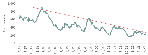
After bottoming at 165,000 tonnes at the end of 2021, inventories rebounded to 300,000 by mid-May, but have since pulled back to 240,000 tonnes. When adjusted for days of consumption, inventories are almost as low as they were back in 2005, just before copper prices more than doubled. In 2005, copper exchange inventories covered consumption by only two days.

By the end of 2021, inventories had fallen to only 2.5 days of consumption, and at 240,000 tonnes today, inventories cover consumption by only 3.5 days — still an extremely low number. Back in 2018, when inventories peaked out at 900,000 tonnes, inventories covered 15 days of consumption.

Copper demand remains strong, supply continues to disappoint, and inventories continue to bump along at extremely low levels. We believe the weakness in copper prices (and all base metals prices) over the last several months represents another great buying opportunity. We see no changes in either the short-term or long-term underlying fundamentals.

Regarding the long-term fundamentals, S&P Global recently published a paper by Dan Yergin titled “The Future of Copper: Will the looming supply gap short-circuit the energy transitions?” The paper garnered significant amounts of press and makes for a very interesting read. The study warns of “unprecedented and untenable” copper shortfalls as suppliers grapple with copper demand that will double by the year 2035. The analysis constructs an extensive “bottom-up” analysis of the impacts of renewable energy given a 45% net reduction in CO2 output by 2035, and net-zero by 2050 (as outlined in the 2016 Paris Accords).

Factoring in traditional copper demand growth from emerging markets like India, S&P Global concludes that copper consumption will double from 25 to almost 50 mm tonnes by 2035. These numbers are truly incredible. Between 2000 and 2020 (a period that experienced surging Chinese demand), copper consumption advanced by 10 mm tonnes from 15 to 25 mm tonnes, or 2.5% per year. Based upon the S&P Global analysis, annual copper demand growth will double — surging from 2.5% to more than 5% per year in the next 13 years.

The study takes an interesting approach to mine supply. S&P Global outlines two scenarios: a “High Ambition” scenario in which copper supply surges but still falls short of demand by 1.5 mm tonnes by 2035 and a “Rocky Road” scenario in which supply falls short of demand by a massive 10 mm tonnes by 2035.

After having studied their report, we disagree with both options: we believe their pessimistic “Rocky Road” scenario is still far too optimistic. S&P Global’s “Rocky Road” scenario assumes copper mine supply and scrap recovery grow from a combined 25 mm tonnes today to 39 mm tonnes by 2035, or by 3.2% per year. By comparison, between 2000 and 2020 mine supply plus scrap grew by only 2.5% per year.

Given the huge depletion problem now gripping the copper mine base and the near total drop-off in new largescale mines (those greater than 300,000 tonnes of copper per year) to be developed over the next 10 years, we believe S&P Global’s expectations are far too generous. Their “Rocky Road” scenario still assumes copper mine plus scrap annual growth will average twice the yearly growth experienced over the last two decades.

Between 2000 and 2020, copper mine supply plus scrap grew 500,000 tonnes per year on average. The “Rocky Road” scenario assumes mine supply plus scrap growth will double to 1 mm tonnes per year between now and 2035. Given our analysis of current supply trends (already painfully obvious in Chile), we believe even the pessimistic “Rocky Road” supply scenario will be impossible to achieve.

We do agree with their assessment that a massive gap is about to emerge between demand and supply that will only get worse as we progress through this decade.

Back in 2016 we wrote a lengthy essay on how investors were completely underestimating the impacts of renewable energy on copper demand: “ To put these figures in perspective, over the last 15 years, copper demand has increased by an average of 500,000 tonnes per year—so renewables have the potential to nearly double annual copper demand. […]

It is unclear how the world will meet these entirely new sources of copper demand. Given that copper mine supply has only grown by about 400,000 tonnes per year over the last 15 years, it is hard to imagine how the copper market can avoid shifting into a large structural deficit over the next several years.”

Back then, copper was at $2.20 per pound and investors were universally bearish. The looming gap about to emerge in copper markets, will not only push prices much higher but will also produce other interesting consequences as outlined by S&P Global:

“The chronic gap between worldwide copper supply and demand projected to begin in the middle of this decade will have serious consequences across the global economy and will affect the time of the Net-Zero initiative by 2050. […] In the 21st century, copper scarcity may emerge as a key destabilizing threat to international security. Projected annual shortfall will place unprecedented strain on supply chains. The challenges this poses are reminiscent of the 20th century scramble for oil but may be accentuated by an even higher concentration of copper resources and the downstream industry to refine it into products.”

We are entering a new copper era. We have discussed extensively how copper markets are about to shift into long-term structural deficit as we progress through this decade. By contrast, the copper analytic community always believed the copper market would remain in structural surplus.

The copper bull market has only started. Copper prices will potentially triple from here. Use the recent weakness in copper prices as a buying opportunity.

A Head Fake in Precious Metals: The Bear Market Drags On

Ever since silver staged a furious catch-up rally back in the summer of 2020 — something that has always signaled a long corrective phase — both gold and silver have been quietly drifting downward. Since reaching their peaks in the summer of 2020, gold prices are now down 15% while silver has fallen more than 35%. Gold and silver equities, as measured by the GDX and SIL ETFs, pulled back over 40% and 50%, respectively.

In our last letter, we outlined the emergence of several important fundamental trends that gave us confidence to say the correction phase in precious metals prices might be ending.

Unfortunately, one of the more important trends, which we thought was flashing a strong buy signal in Q1 has reversed. In past letters, we have discussed how the gold bull market’s next leg would be driven by western investors, not by eastern investors as was the case in the huge gold bull market between 1999 and 2011. We follow 16 publicly traded ETFs that invest in physical gold, to track the interest of western investors, which has now turned decidedly bearish.

After aggressively accumulating almost 1,500 tonnes of gold between Q4 2018 and Q3 2020, our 16 ETFs spent the next 18 months liquidating almost 450 tonnes of gold or 12% of their holdings. The gold price peaked in August 2020 just as our 16 ETFs swung from accumulation to physical shedding. We believe gold selling from these ETFs produced the 15% pullback since September 2020.

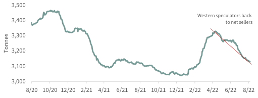
In January, our physical gold ETFs swung from shedding to accumulating gold. From mid-January to the beginning of April, these ETFs accumulated almost 260 tonnes, approximately 60% of the gold they liquidated over the previous 18 months.

Given the surge in both inflation and geopolictical tension initiated by Russia’s invasion of Ukrainian, we thought we had entered into a new phase of western accumulation and conjectured that prices would rise. However, starting in mid-April, the ETFs swung back again to being gold liquidators. Rising short-term interest rates produced a 10% surge in the trade weighted value of the US dollar whose strength has more than overcome spiking inflationary expectations and global tensions.

The accumulation behavior of the 10 physical silver ETFs we track has been even more bearish. Liquidations ended mid-January and our silver ETFs experienced a brief period of accumulation. However, by the end of February, the ETFs had returned to aggressively shedding silver. By mid-July, they had shed over 1,000 tonnes. Again, the strong dollar has more than overcome rising inflation and global tensions.

At the end of Q1, we thought westerners had turned from sellers into precious metals buyers, however, the recent behavior in gold and silver ETFs tell us we were wrong. Given the Fed has strongly stated its intension to continue raising short-term rates, and given the continued upward momentum in the dollar, it looks like the western investor has again adopted a bearish stance. The nearly two-year corrective phase in both gold and silver prices has yet to run its course.

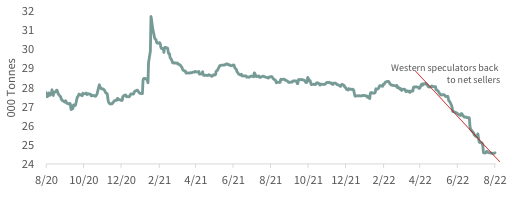
Also lending credence that the corrective phase in both gold and silver is not yet over is the behavior now being exhibited by gold traders in the COMEX futures market, although the behavior of silver futures traders is about to flash a potential buy signal.

Over the last 20 years, several significant buy signals have been given when commercial gold and silver traders positioned themselves net long and speculative traders went net short. For those who study the positioning of traders in various commodity markets, the “commercials” (i.e., those who use the futures markets to hedge various commercial needs) represent the “smart money.” “Speculators” (i.e., hedge funds, algorithmic traders, and other trend-followers) represent the “dumb” money.

Whenever smart money goes net long and dumb money goes net short, that often coincides with a significant bottom in precious metals. It doesn’t happen very often, but when it does, there is a significant buying opportunity.

The last time gold and silver commercial traders were long and speculators were short for long periods was back in the late 1990s / early 2000s. Given that gold and silver were incredibly cheap and investors were incredibly bearish (because of the torrent of central bank gold selling), it not surprising that the net long positioning of commercial and net short positioning of speculators for almost four years was telling you that gold represented the buying opportunity of a lifetime. If you had bought gold during these four years, you would have vastly outperformed both the bond and stock markets.

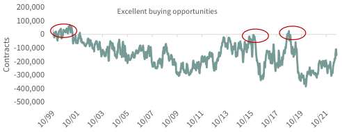
Since the massive gold bear market bottom made back in the early 2000s, the instances of commercial traders going long and speculators going short have been few and far between. As you can see, commercial and speculators almost went net long and net short at the end of 2015 just as gold was ending its 45% pullback from its 2011 highs. With gold trading below $1,100 per ounce, that again turned out to be an excellent buying opportunity.

The final instance when gold and silver commercials went net long and speculators went net short occurred back in August 2018. With gold trading below $1,200 per ounce, the positioning of smart and dumb money again gave a great buy signal. Over the next 2 years, gold prices surged over 75%.

Today, the positioning of commercial and speculative gold futures traders is not anywhere close to flashing a buy signal. Even though commercial traders have cut their net short exposure by almost 50% in the last three months, they remain significantly net short. Speculative traders also cut their net long exposure by 50% in the last three months, but they remain 125,000 contracts net long.

Trader positioning in the silver futures market has become far more interesting in the last several months. As you can see from the chart below, commercials have slashed their net short position by almost 90% over the last three months.

As silver has pulled back, commercials are on the verge of going net long. As of today, they are only net short 9,600 down from almost 70,000 contracts back in April. Silver market speculators have also significantly cut back on their net long position. As silver has pulled back, speculators have become much less bullish and have cut their net long position from over 50,000 contracts to only 5,400 today—a drop of almost 95%. And just as silver commercial players are on the verge of becoming net long, speculators are on their verge of going net short — a sign that the two-year corrective phase in silver is coming to a close.

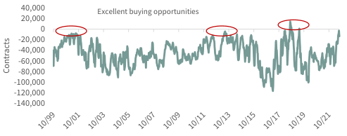
The silver futures market is about to flash a significant buy signal; however the gold market still has not. For those who want to time the ending of the corrective phase in both gold and silver markets, we recommend waiting for commercial to go long in both and for speculators to go net short before significantly increasing their precious metals exposure. When this happened back in August 2018, it turned out to be a great time to significantly increase precious metals exposure.

On the positive side, we should mention that the ratio of gold to oil has flashed another buy signal. When gold gets expensive relative to oil (an ounce of gold buys 30 barrels or more), oil related investments have historically strongly outperformed gold investments.

Conversely, when gold gets cheap relative to oil (an ounce of gold buys only 15 barrels or less of oil), then gold related investments have strongly outperformed oil related investments. The last time the gold-oil ratio hit 15 was back in September 2018 (the exact time that COMEX traders had flashed a huge buy signal) when gold traded down to $1,175 and oil prices hit $80. For the next two years, gold and gold related investments radically outperformed oil and oil related investments.

After bottoming in September 2018, gold rose 75% and gold related stocks rose 125%. Over the same two-year period, oil went negative, and oil related equities fell over 60%.

Back on March 8, with oil spiking to $130 per barrel and gold trading down to $1,980, the gold-oil ratio touched 15 intraday, the same level we saw back in September 2018. On June 14, we got another buy signal on the gold-oil ratio. With oil trading at $124 per barrel and gold trading down to $1,805 per ounce, the gold-oil ratio touched 14.6, again in line with the level back in September 2018.

The only difference was that in 2018 the gold-oil ratio buy signal was confirmed by strong buy signals in the positioning of gold and silver COMEX traders as just described above, which has not happened yet.

Given that we have now been given two precious metals buy signals from the gold-oil ratio, the only thing missing from that September 2018 set-up will be the bullish signal flashed from COMEX gold future traders. Will we get a buy signal in the next several months? We are heading in the right direction, and we will carefully monitor their position as we progress through Q3.

Precious metals have now been through almost two years of corrective price action and it has paid handsomely to have minimal exposure over the last two years. Having minimal exposure to investments in the precious metals areas has been a huge positive input to performance over the last two years. However, given that we are strong believers that huge gold and silver bull markets sit directly in front of us, we are carefully monitoring both markets for strong buy signals.

Given the recent pullback in all precious metals investments in the last three months, we have used this weakness to add to our precious metals exposure, however we have now paused before we increase our exposure again.

Nuclear Sentiment Continues to Improve

The pendulum continued to swing in favor of nuclear power during Q2. The Russian invasion of Ukraine has put national energy security front and center while the limitations of wind and solar (namely their intermittency) are becoming acutely appreciated. We have long argued that nuclear power remains the only source of high EROEI carbon- free baseload power. Policy makers are beginning to take note.

The European Union ratified its Green Taxonomy, officially labeling nuclear power as part of a carbon-free future. The Taxonomy was approved on a preliminary basis last July but subject to a final ratification. The proposal was extremely controversial with many countries, led by Germany, advocating against the inclusion of nuclear power in a green future. The ongoing energy crisis throughout Europe seems to have outweighed any opposition.

France, the UK, the Netherlands, and even Japan are embarking on new nuclear buildouts or extensions of existing facilities. Even Germany, which has spent the past decade dismantling its nuclear power capacity, is talking about building new reactors.

So-called Gen IV reactors (often referred to as “small modular reactors”) continue to gain traction. NuScale Power, a company pursing a new reactor design, pursued a public listing as part of a de-SPAC process and sports a valuation more than $3 bn. We have started an extensive due diligence process on several new Gen IV reactor designs and are intrigued by some of them. We believe some of the new designs could help to greatly reduce costs, improve safety, and lower the volume of radioactive waste by nearly an order of magnitude – the three main pushbacks against nuclear power.

As we go to print, the Inflation Reduction Act of 2022 has just been signed into Law. Included in the Act is a little mentioned but highly impactful appropriation for existing nuclear power plants. The Act calls for $30 bn in credits for current operations by providing for a “Zero Emission Nuclear Power Production Credit.” According to Bloomberg, analysts believe this incentive could help keep nearly 40% of the current US nuclear power capacity operational going forward.

Furthermore, the bill calls for an advanced reactor production tax credit and investment tax credit which will directly benefit the development of new Gen IV reactors. Lastly, $700 bn has been provided for the support of high-assay low-enriched uranium production (HALEU). Most Gen IV reactor designs utilize HALEU which is simply uranium that has been enriched to 17-20% instead of the normal 5% for current nuclear reactors (for context, weapon grade uranium has been enriched to 90%). There has been concern over the availability of domestically produced HALEU, particularly since the only source of the material presently comes from Russia.

Public sentiment is clearly shifting in favor of nuclear energy. We continue to believe that nuclear energy is the ideal solution to our energy needs – it is both extremely efficient, with a record-setting EROEI of 100:1 and produces no carbon. We commend policy makers for finally realizing these benefits.

The Temporary Respite in the Agricultural Crisis Won’t Last

Grain prices pulled back sharply in July on news that Russia would allow Ukrainian grain exports to resume via the Black Sea. Since the end of February, all Ukrainian grain exports through Black Sea ports have been blockaded by the Russian Navy. The resumption of Ukraine’s grain exports is of huge short-term importance. Ukraine wheat and course-grain exports represent a significant percentage of global seaborne grain trade—approximately 11%, and their blockage put significant additional upside pressure on grain prices in the first six months of 2022.

Putting aside the many dangers still involved in the exporting of Ukrainian grain (Russia began an aggressive shelling campaign of Odessa literally the day after the grain export deal was signed), the resumption is of extreme importance to a world suffering huge shortages. Even though grain exports have resumed, war-related pressures are creating large problems for Ukrainian agriculture that will continue to impact world grain balances well into 2023.

Because of extensive war-related field damage, shortages of fertilizer, diesel fuel, and manpower, the USDA , in its most recent “World Agricultural Supply and Demand Estimates” (WASDE) projects that Ukraine’s 2022 wheat crop will fall from 33 mm tonnes harvested in 2021 to only 19 mm tonnes this year—a drop of 14 tonnes or 40%. Course-grains (corn, soybean, sorghum, barley, oil, and other oil seeds) will fall from 54 mm tonnes harvested in 2021 to only 32 mm tonnes harvested this year—a drop of 22 mm tonnes.

Combined wheat and course-grain production will fall by 36 mm tonnes. The drop in harvest size this year will result in large impacts to global export markets for at least next 12 months. Last year Ukraine exported almost 50 tonnes of wheat and course-grain, representing 11% of those markets. For the coming 12 months, the USDA projects that Ukraine will only export only 20 mm tonnes of wheat and course-grain—a drop of 30 mm tonnes, approximately 60%. A drop of this magnitude will keep both wheat and course- grain markets tight until the 2023 harvest comes in next fall.

Even before all the Ukrainian problems erupted this spring, problems in the 2021 growing season were already putting pressure on grain prices. Last summer, both corn and soybean prices almost made all-time highs — long before problems emerged in the Ukraine. Weather-related problems, primarily from severe drought conditions in Brazil, forced the USDA to reduce their 2021-2022 crop year forecast for global corn and soybeans supply by 45 mm tonnes — a significant reduction of 3%.

This year weather conditions are again shaping up to be even more challenging. In India, a spring heat wave severely damaged India’s winter wheat crop. In 2021, India harvested almost 110 mm tonnes of wheat and exported 8 mm tonnes — representing 4% of the global export market. Because of heat-related damage, it looks like India’s wheat crop will come in under 100 mm tonnes, down 10%. Three months ago, to bring down wheat prices, India banned all wheat exports—a prime example of “food nationalism,” a subject we discussed in our last letter.

Severe heat and drought are also gripping huge swaths of Europe and the UK. The European Union (EU) has dropped its 2022 yield assumptions for soybean, corn, and sunflower production by 10%. The EU is the world’s largest wheat exporter, representing almost 17%, and they represent 6% of export trade in course-grains. A 10% drop in yields will add significant tightness to global grain markets that are already significantly tight.

In the United States, we believe both corn and soybean yields are at risk for significant reductions as well. Extremely hot weather conditions have now existed for weeks in the both the corn belt and in prime soybean growing areas, just as both crops pollinated. Extreme heat and crops that were planted up to 2 weeks late could produce a significant negative impact on both corn and soybean yields.

Regarding corn, US farmers reduced their 2022 corn plantings significantly in favor of soybeans, most likely driven by extreme high nitrogen prices (soybeans, being a legume, do not need nitrogen fertilizer application). US farmers planted almost 4% less corn acres this year and the USDA assumes corn yields will equal last year’s record of 177 bushel per acre. Even with record yields, the USDA predicts 2022/2023 corn ending stocks will reach 1.47 bn bushels—approximately in line with the 30-year ending corn stock average.

However, any drop in corn yield will produce huge tightness in the US corn market. If yields were to fall to 171 bushels per acre—the realized yield in 2020, ending stocks would fall to 970 mm bushels; a level not seen since the 2012 drought in which corn yields plunged to 122 bushel per acre.

Regarding soybeans, farmers wound up planting approximately 1 mm additional acres this year versus 2021, although this turned out to be 1.2 mm less than USDA estimates published back in May. Even with an estimated yield assumption of 51.5 bushels per acre (up slightly from last year’s soybean yield of 51.4, but not too far off form 2016’s record soybean yield of 51.9) the USDA projects soybean’s 2022/2022 ending stocks to only reach 230 mm bushels — extremely low.

Soybeans are priced only 60 cents below their all-time high prices reached back in the 2012 drought year and again in June. Because of extremely low projected ending stocks, any reduction in soybean yields will put extreme upward pressure on prices. If soybean yields fall to 49.9 bushels per acre — the average soybean yield over the last five years — ending stocks would fall to only 90 mm bushels — the lowest level ever seen in US soybean markets.

Although Ukraine’s return to the global grain trade has put short downward pressure on markets, we believe the global agricultural crisis which began to emerge last summer is far from over. Volatile and challenging weather conditions experienced over the last several years will continue to only get worse as we progress through this decade.

Last year’s extremely challenging weather conditions (especially in Brazil) severely impacted global corn and soybean supply, adding significant upside price pressure last year. War-related stress continues to have huge impacts on Ukraine’s agricultural activities and now unfavorable weather conditions in Europe will added further stresses to grain supply. Also, we believe that big weather-related reductions to US corn and soybean yields will add additional supply worries to global grain markets.

High fertilizer prices also continue to be a huge problem for farmers. Across Asia and Africa stories are plentiful of farmers unable to apply standard quantities of fertilizers because of high prices. Fertilizer under-application, especially in the third world, will be another factor causing yield disappointment to this year’s grain supply—a subject that is hard to quantify and is poorly understood by most analysts.

Finally, new forces are at work creating unforeseen consequences for global agriculture markets as we progress through this decade. Because of poorly thought-out government policies, global agricultural markets have now become highly integrated into global energy markets.

Nothing better demonstrates this phenomenon than the US corn and soybean markets over the last 15 years. Almost 40% of the corn crop is now processed into ethanol and 25% of the soybean crop is now used to make bio-diesel. The worse the global energy crisis becomes the bigger the demand will be for bio-fuel production, resulting in further upward pressure to grain prices.

We believe the global agricultural crisis has just started and will run for many years with many unexpected twists and turns. We continue to recommend significant exposure to agricultural related equities.

---

Original Post

Editor’s Note: The summary bullets for this article were chosen by Seeking Alpha editors.