EWMA: Simpler And Better Equity Statistics (Technical Analysis)

The Legend

How To Make A Stochastic Volatility Supermodel and Use 3D Volatility Ratios For Investment Decision Making discussed the EWMA Volatility (standard deviation) calculation in some depth.

EWMA = Exponentially weighted moving average

EWMA numbers are superior in every way to those produced by the classical statistical equations which are based on fixed time segments. 3D Volatility made the bold claim that this view is close to an academic consensus in Finance.

My guess is that EWMA is not universally used for equity portfolio and risk analysis because the astounding simplicity of the calculation is not widely understood . Coding EWMA is about as complicated as doing a running total. On the basis of simplicity and accuracy, EWMA is possibly a refutation of the traditional statistical variance and covariance formulas.

The Plan

Everyone has a plan until they get punched in the mouth.

Mike Tyson

After almost 50 years of experience, I’ve noticed that it is usually a good idea to start with at least a vague plan. The idea is to analyze the effect of volatility on equity return. The graphic below shows what I think are the minimum data elements needed to analyze QQQ.

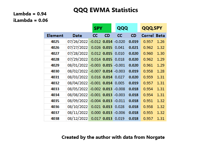
CC= Close to Close = Logarithmic daily return

CD = Close deviation = EWMA standard deviation, using the Lambda parameter of 0.94. iLambda = 1 – Lambda = 0.06. Lambda controls measurement sensitivity. Many PhD theses could be written on Lambda selection of course, here we will use 0.94.

Standard deviation is a variance calculation. Variance = CC^2 (CC Squared). 3D Volatility explained the EWMA variance -> CD calculation.

Correlation and Beta are calculations needing a covariance in addition to the variance.. Covariance = CCSPY * CCQQQ.

I think the easiest way to understand EWMA is to understand the calculation given here first and then watch a YouTube EWMA video or two, or five, which generally do a decent but awkward and incomplete job of proving that the logic shown here is correct. Without discussing the correct calculation methodology, the videos are confusing and misleading.

This article will show how to quickly and easily calculate covariance. The capability of EWMA to handle covariance is theoretically important because it strongly suggests that the EWMA model is a viable replacement for classical variance and covariance formulas for equity analysis.

The Gettin’ Place

Carla Jean Moss: Where’d you get the pistol?

Llewelyn Moss: At the gettin’ place.

No Country For Old Men

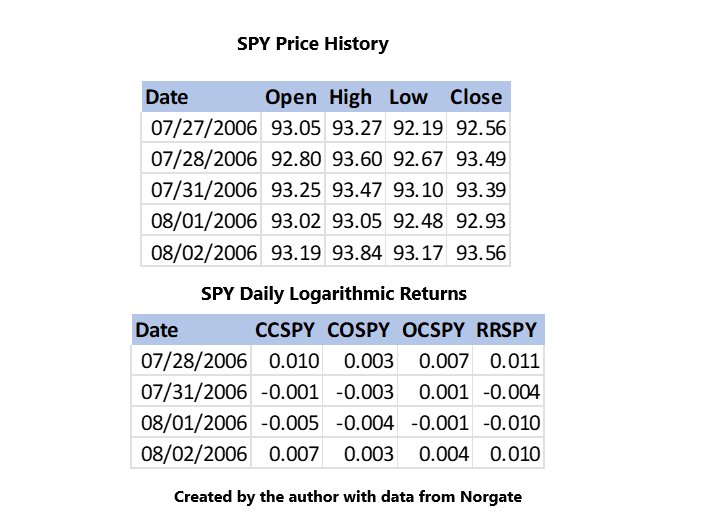
I’d like to think that the time I’ve spent learning the intricacies of downloading price history has ultimately made me a better person. Price history should be accurate and dividend adjusted. Around 2015, I made the major strategic decision to code my own indicators. Usually Norgate runs as a front end to software that has built in indicators, but the basic info above is fine with me.

My thought process was; if I’m too dumb to code an indicator, what are my chances of being able to interpret it properly.

Daily prices are converted/normalized into logarithmic returns.

CC = Close to Close

CO = Open to Close

OC = Close to Open

CC = CO + OC

The first day of the sample always gets dropped.

CC is needed for the CD covariance calculation.

A Little Techno Shade

Price history data elements can be used, as is, to make a price chart. A chart is undeniably a better way to visualize the raw data than say, manually scrolling through the numbers.

Despite being easy to build and useful, price charts are logically flawed because the data normalization issue has not yet been resolved. The non-normalized structure practically limits the analytical usefulness of the underlying data because it is more difficult to interpret in that state. This is an important reason why, in the broad discipline of time series return analysis, technical analysis is typically not seen as one of the sharper tools in the shed.

The technique shown here seems to be the simplest and most efficient way of normalizing return data.

EWMA Covariance

3D Volatility showed the CD variance -> deviation calculation. Covariance calculation logic is exactly the same except instead of the variance theme of x^2, covariance does x * y.

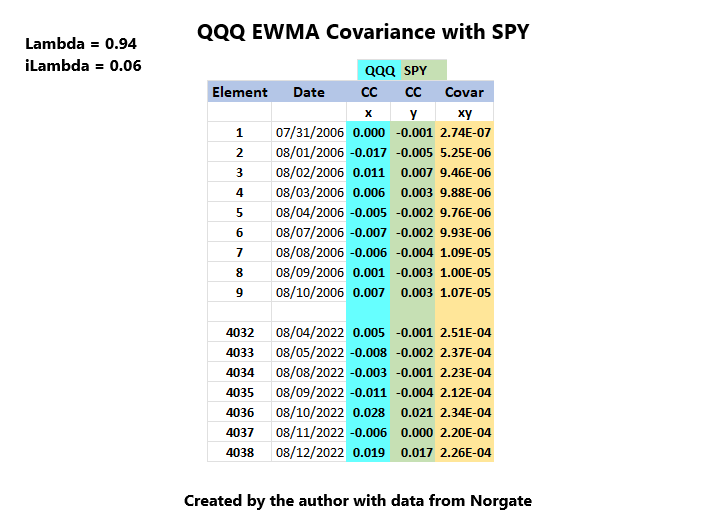
The first element of Covar = xy or CCQQQ * CCSPY.

The rest of the numbers are calculated in an identical manner. i = Element:

For i = 2 to 4038

Covar(i) = (CCQQQ(i) * CCSPY(i) * iLambda) + (Covar(i-1) * Lambda)

Next i

Correlation and Beta

Once Covariance and Variance have been determined, Beta and Correlation are straightforward to calculate.

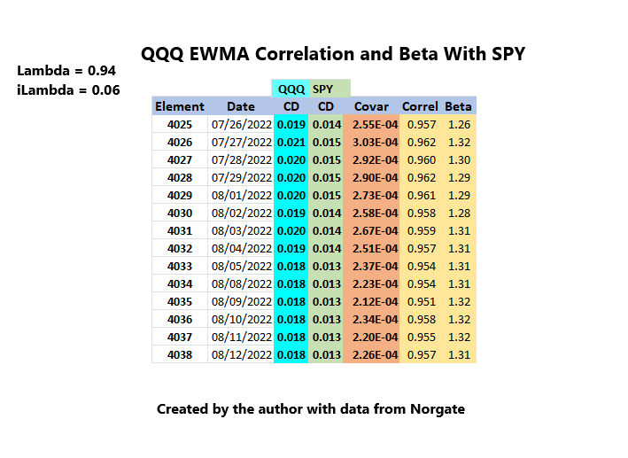
There is no longer a need for CCSPY and CCQQQ. But now CDSPY and CDQQQ come into play. The calculations go something like:

For i = 2 to 4038

Correl(i) = Covar(i) / (CDQQQ(i) * CDSPY(i))

Beta(i) = Covar(i) / CDSPY(i)^2

Next i

EWMA Pedagogical Issues

The calculations described above produce totally accurate statistics for every day in a time series except the very earliest in less time than the classical calculation requires to generate statistics for a single day (give or take).

The pedagogical problem is that when you run this by someone that knows classical statistics they will typically, initially find it unbelievable because the handling of Variance and Covariance is so different.

I had a theory that all the guys that do EWMA YouTube videos know the subject matter is difficult to grasp. Since their presentations are all the same, maybe there is some accepted pedagogical methodology they all know to get students through this trauma. That sort of explains the excessive time they spend discussing how to prove the simple routines outlined above.

With a little work, the generic YouTube EWMA examples can be used to prove that the given calculation techniques are accurate. What the videos don’t point out, is that the examples they give are far from acceptable coding solutions, assuming the developer has any self respect. In addition to being horribly ugly and inefficient, the implied methodology is close to unsound.

My original sense was that the presenters know the streamlined calculations because they’re just elementary exponential moving average theory. On the other hand, one has to wonder why they don’t give any clear indication that they have the slightest clue about the simplicity and elegance of the correct solution.

EWMA Theoretical Importance

There are probably excellent reasons to say not so fast, but the efficiency and accuracy of EWMA raises significant questions about the correctness of the classical variance and covariance equations. With an EWMA solution for both variance and covariance, from an Occam’s razor perspective, arguments for the classical calculations seem feeble.

EWMA seems to be the most important development in modern statistics since 1900. There is absolutely no surprise that the concept is easiest grasp through an information theory perspective.

Research Possibilities

Return analysis with EWMA offers vast possibilities for important research. Any shakiness in the classical equations will likely lead to a reassessment of the current dubious academic understanding of high dimensionality which is dismissed as noise.

Summary Of New Daily Measurements

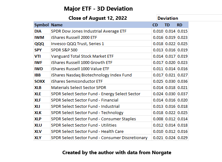
Supermodel and 3D Volatility define a three dimensional EWMA volatility structure all based on logarithmic return numbers.

CD = Close Deviation <- CC^2

TD = Toltec Deviation <- (Abs(CO) + Abs(OC)) ^2

RD = Range Deviation <- RR^2

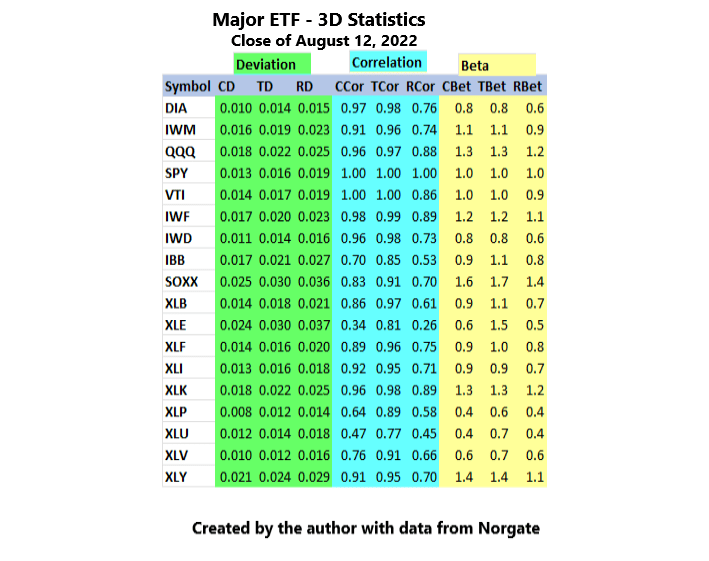
EWMA covariance now gives us Correlation and Beta.

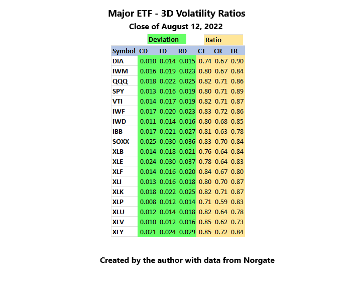
Volatility Ratios were introduced in 3D Volatility. Volatility ratios have a normal return distribution, possibly making them theoretically important.

CT = CD/TD, median = .80

CR = CD/RD, median = .67

TR = TD/RD, median = .84

The medians are based on SPY, but they don’t change much between different equities.

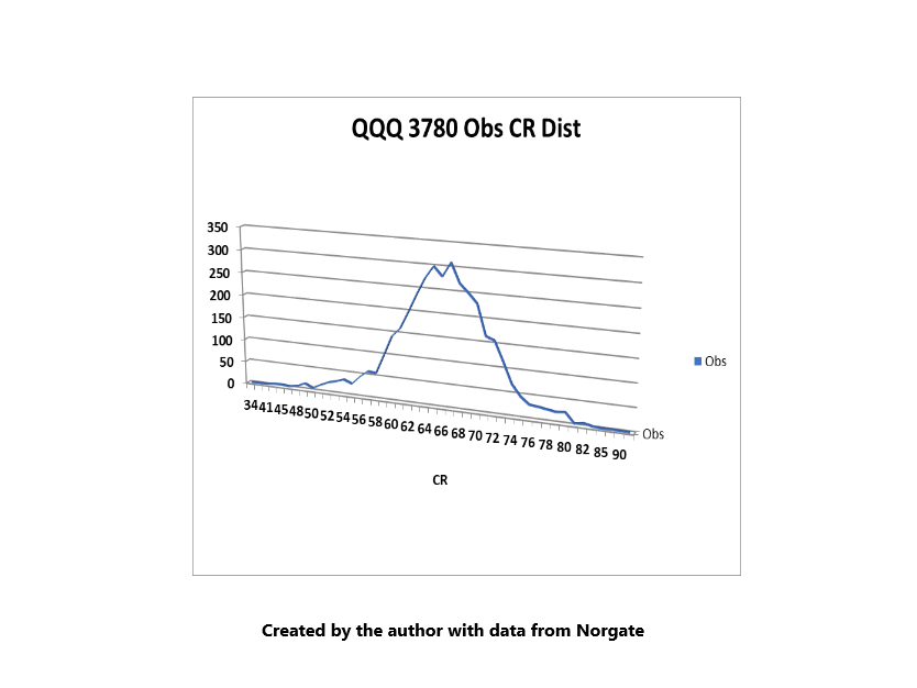
3780 trade days is 15 years, beginning on 8/9/17.

The normal looking bell shaped curve seems to be consistent across all reasonable timeframes.

The distribution uses a binning technique of multiplying the ratio by 100.

Current QQQ CR = 0.71 which is 71 on the horizontal axes. Getting a bit close to the right tail at the 85th percentile.

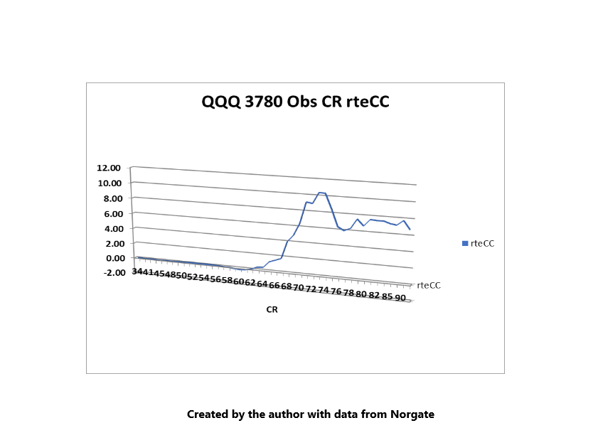
Return peaks at 0.74. If the recent rally continues at its July strength (for example), this ratio will increase because closes will tend to be high within the range. It goes without saying, that this daily number is useful to keep an eye on.

The 10 means that an investor who held QQQ at CR 74 and below made 10 times their investment, versus 6.71 times for buy and hold.

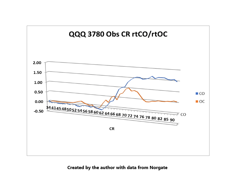
CO and OC returns are easier to visualize with natural logs. The clear suggestion is that it’s OK to hold QQQ CO at higher CR ratios, but OC tends to get problematic.